

1. Introduction
Himalayan and Trans-Himalayan glaciers are characterized by the presence of debris in the ablation zone of the glacier (Fujii and Higuchi, 1977; Benn et al., 2012; Bolch et al., 2012). Large valley walls and steep headwalls are the source of debris (Kraaijenbrink et al., 2017), which alters terminus dynamics (Scherler et al., 2011) and ablation of the underlying ice by altering the surface energy balance and imposing a barrier between the atmosphere and ice (Nicholson and Benn, 2013). Debris-covered glaciers are an important source of water for hydro-electricity generation, irrigation, and consumption. Future water availability in the Himalayas is dependent on the snow and ice cover. Recent changes in climate have caused the loss of glacial area and changes to snow cover in the Himalayan region. Debris-covered glaciers have lost significant mass in recent decades despite the thick debris (Bolch et al., 2008, 2011; Kääb et al., 2012). Most of the melting of ice beneath the debris resulted in the expansion of existing glacier lakes (Gardelle et al., 2011; Byers et al., 2013) and formation of several large supra-glacial ponds (Qiao et al., 2015) at the surface of the debris-covered glacier.
In general, debris thickness ranges from a few millimeters to meters. Debris thickness greater than approximately 0.02 m retards melting (Östrem, 1959; Fujii, 1977; Mattson et al., 1993), however, the critical thickness at which this occurs varies for each glacier and seems to be controlled by thermal properties of the debris (Reznichenko et al., 2010). The melt rate beneath the debris depends on debris thickness (Rounce and McKinney, 2014) and determined by atmospheric conditions, thermal coductivity, porosity, moisture within the debris, albedo, and surface roughness (Juen et al., 2013). Heat transfer might occur by conduction, radiation or convection, however, conduction is the primary mode of heat transfer from surface of the debris to the debris/ice interface (Östrem, 1959), especially deeper than about 0.2 m (Conway and Rasmussen, 2000). Thermal conductivity has a significant role in ice melt (Nakawo and Rana, 1999) and is increased when the amount of water content is high (Juen et al., 2013) as pore spaces filled with air have a lower thermal conductivity than pores filled with water. Thermal diffusivity is a combination of thermal conductivity, density and specific heat capacity and is another important property of the debris that determines how the temperature within the debris varies when the temperature changes at the surface (Juen et al., 2013). The mean value of thermal conductivity in combination with meteorological variables can estimate ice melt underneath the debris layer with sufficient accuracy (Shahi and Kayastha, 2015). Similarly, researchers have found the effect of supraglacial debris on glacier melt using a surface energy balance model with surface temperature and meteorological variables (Nakawo and Young, 1982; Conway and Rasmussen, 2000; Kayastha et al., 2000; Takeuchi et al., 2000; Han et al., 2006; Nicholson and Benn, 2006; Reid and Brock, 2010; Reznichenko et al., 2010; Chand et al., 2015). Fujita and Sakai (2000) also found that storage and release of heat from the debris changes the surrounding air temperature, which varies over time and season. However, studies focused on the role of thermal properties in ice melt beneath the highly heterogeneous debris are still lacking in case of the Nepalese Himalayas. This paper presents the thermal regime of supraglacial debris on a Lirung debris-covered glacier, Central Nepalese Himalaya. Thermal properties for two different sites in three different seasons of 2013 and 2014 are presented. Positive degree-day factors were also derived from the observed air temperature and ice melt from the glacier.
2. Study area
This study was conducted on Lirung Glacier (28.422°N, 85.517°E) in the Langtang catchment of Langtang Valley located in the Central Nepalese Himalaya (Figure 1). The elevation of this glacier ranges from 4,000 m a.s.l. at the terminus to 7,234 m a.s.l. at the peak of Mt. Langtang Lirung. Lirung glacier boundary was obtained from the International Centre for Integrated Mountain Development (ICIMOD) glacier inventory (Bajracharya et al., 2014). Further processing of the glacier extent was carried out using ASTER DEM 2009 of 30 m resolution downloaded from http://gdex.cr.usgs.gov/gdex/ and Sentinel 2A image of October 15 2017, obtained from the Copernicus open access hub. The Lirung catchment covers about 13.51 km2 of which 5.34 km2 is clean ice, 1.14 km2 is debris-covered and 6.03 km2 is covered by exposed rock. The present study focuses only on the lower debris-covered portion of the glacier, which accounts for 18% of the total glacier area. The elevation of this debris-covered area ranges from 4,000 to 4,400 m, has a gentle slope relative to the accumulation area, and is covered with debris that ranges from a few cm to greater than 1 m. Most of the debris-covered area (about 71%) has a slope less than 10° and a southern aspect (about 61%). This zone has already detached from the clean part of the glacier. Below the debris-covered glacier is a pro-glacial valley with a large pro-glacial pond. From this pond, the melt water flows out as Lirung River, a small river which ultimately joins the Langtang River in the down valley.
Figure 1

Figure 1 (a) Geographic context of the study area within Nepal; (b) The Lirung catchment, with the Lirung debris-covered glacier showing the location of thermistors, ablation stakes, and AWS. Backdrop is Sentinel-2A false-color composite from October 15, 2017
3. Datasets and methodology
3.1. Datasets
Datasets include temperature measurements from different debris thicknesses to obtain information about the debris internal temperature profiles. Two sets of thermistors were installed at two different sites, i.e., one at the AWS site, where the debris thickness was 0.38 m during the monsoon season and 0.4 m during the winter and pre-monsoon season, and one above AWS, where debris thickness was 0.42 m during the monsoon season and 0.4 m during the winter and pre-monsoon season (Table 1). The two sites in the monsoon season were randomly chosen at two different elevations (Table 1) without giving consideration to the debris thickness. However, a debris thickness of 0.4 m was desired at both sites in the winter and pre-monsoon seasons. The installation site of thermistors in each season was kept the same except during the monsoon season. The thermistor position at site 2 during the monsoon season was about 35 m lower elevation than the thermistor position during the winter and pre-monsoon season. We manually excavated the debris down to the debris/ice interface and measured the debris thickness and a set of thermistors with three sensors were installed at various depths within the debris from the surface (0 m) to debris/ice interface (Figure 2). The ice was then covered with excavated debris. Temperatures were recorded for 13 days at each site using a DVT4 Supco SL300/400 series sensor. Measurements were carried out in three different seasons of 2013 (monsoon from September 20 to October 3, winter from November 29 to December 12) and 2014 (pre-monsoon season from April 6 to April 19). The temperature at the surface of the debris was measured by inserting a thermistor within a few millimeters of the debris to avoid direct heating of the sensor by solar radiation. Temperatures were recorded at every 5 minutes and averaged to obtain hourly data. Debris composition includes clast-supported cobbles near the surface (up to 0.1 m) and was dominated by soil, silt, and sand at greater depths at each site and each season. Moisture content at the AWS site was slightly higher than the above AWS site which was observed visually during the monsoon season. Temperatures at each site and in each season were stabilized within two days of installation and hence dataset from day 3 were considered for analysis. Temperature sensors failed to record temperatures at site 1 from September 20 to September 22 due to losing connection with the data logger. Therefore, we used dataset from September 25 onwards only for this site. Initially, temperature sensors were installed at the surface (0 m), 0.2 m, and 0.4 m at both sites in the winter season. However, temperature differences between sensors installed at 0.2 m and 0.4 m was negligible, therefore sensors installed at 0.2 m were changed to 0.1 m from the surface on December 5. Air temperature at 1 m above the debris-covered surface was measured using a Vantage Pro2TM sensor (28.23269°N, 85.55919°E, and 4,093 m a.s.l.). Similarly, ablation measurements were carried out on a daily basis over the measurement period using ablation stakes made of bamboo at different thickness of the debris that ranged from 0.003 m (black-coloured ice (dirty ice)) to 0.42 m and at different elevations (4,070–4,157 m) (Table 2) during each season. We used 7 stakes during the monsoon period and 5 stakes during the winter and pre-monsoon period.
Table 1 Position of the thermistor sensors in each season and their respective elevation on the glacier
| Elevation (m a.s.l.) | Monsoon (2013) | Winter (2013) | Pre-monsoon (2014) | |||||
| Site 1 | Site 2 | Site 1 | Site 2 | Site 1 | Site 2 | |||
| 4,093 | 4,156 | 4,093 | 4,196 | 4,093 | 4,196 | |||
| Depth from surface (m) | 0.1 | 0.05 | 0.0 | 0.0 | 0.0 | 0.0 | ||
| 0.2 | 0.15 | 0.1 & 0.2 | 0.1 & 0.2 | 0.1 | 0.1 | |||
| 0.3 | 0.35 | 0.4 | 0.4 | 0.4 | 0.4 | |||
| Total debris thickness (m) | 0.38 | 0.42 | 0.4 | 0.4 | 0.4 | 0.4 | ||
Figure 2

Figure 2 Supco thermistors installed at three different debris thickness (0.0 m, 0.2 m, and 0.4 m) in the winter season. The left panel shows the position of the thermistor at the AWS site and the right panel shows the position of the thermistor above the AWS site
Table 2 Ablation stakes used for ice melt measurements at different debris thickness and elevation of the glacier in different seasons
| Stake No. | Season | Debris thickness (m) | Elevation (m) |
| 1 | Monsoon and pre-monsoon | 0.003 (Dirty ice) | 4,097 |
| 2 | Winter | 0.02 | 4,095 |
| 3 | Monsoon, Winter and Pre-monsoon | 0.05 | 4,070 |
| 4 | Monsoon and winter | 0.10 | 4,070 |
| 5 | Pre-monsoon | 0.16 | 4,094 |
| 6 | Monsoon and pre-monsoon | 0.20 | 4,093 |
| 7 | Winter | 0.23 | 4,136 |
| 8 | Monsoon | 0.25 | 4,157 |
| 9 | Winter | 0.28 | 4,109 |
| 10 | Pre-monsoon | 0.35 | 4,154 |
| 11 | Monsoon | 0.38 | 4,093 |
| 12 | Monsoon | 0.42 | 4,154 |
3.2. Methodology
3.2.1. Thermal conductivity and thermal diffusivity
The effective thermal conductivity, ke, of the debris was determined following the methods of Nicholson and Benn (2013), Hagg et al. (2014), and Rounce et al. (2015), which is given by
where c is the specific heat capacity (J/(kg·K)) of the debris material, ρ is the bulk density (kg/m3) and α is the thermal diffusivity (m2/s) of the debris. Standard values of density (2,700 kg/m3), specific heat capacity (750 J/(kg·K)) for rock were assumed (Conway and Rasmussen, 2000) and a bulk porosity of 0.33 was assumed to obtain the volumetric heat capacity of the debris (Nicholson and Benn, 2013). ke is directly proportional to (α) of the debris. α is an important thermal property of debris and is inversely proportional to the amount of heat that is necessary to cause a temperature change in the material and it depends upon the density and specific heat capacity of the debris. α was derived by the method of Conway and Rasmussen (2000) using a one-dimensional thermal equation:
where T is debris temperature, t is time, and z is debris depth from the surface. The gradient of the line of best fit between the first derivative of temperature with respect to time and the second derivative of temperatures with respect to depth approximates α. Temperature measurements in regular depth intervals are needed at a minimum of three different positions to estimate the depth-averaged thermal diffusivity using the Conway and Rasmussen (2000) method (Juen et al., 2013). In our study, only temperature measurements at the site of AWS during the monsoon season (September 24 to October 3) and both sites during the winter season only for 4 days (December 1 to 4) met this criterion. We chose only AWS site from the winter season to make a better comparison with the monsoon season and therefore, α was estimated only for the AWS site for both seasons.
3.2.2. Degree-Day factor (DDF)
DDF (mm/(°C·d)) is the ratio of glacier melt and the positive accumulated temperature over the measurement period (Equation (3)) (Kayastha et al., 2000). Data from ablation stakes and daily air temperature for three different seasons were used to estimate DDF.
where A is the ablation during the measurement period (mm), and PDD is the positive accumulated temperature (°C) at the AWS site. Ablation stakes were measured from September 22 to October 3, 2013, November 30 to December 12, 2013 and April 6 to 16, 2014 for the monsoon, winter and pre-monsoon seasons, respectively. The same time periods were used to measure the cumulative positive air temperature for each season to estimate DDF. We used temperature data that was measured at 4,093 m a.s.l. for each ablation stakes at different elevations.
4. Results
4.1. Debris temperature profiles in different seasons
Temperature measurements revealed that average surface temperature (−1.77 °C) was cooler than average air temperature (−0.15 °C) in the winter season, while in the pre-monsoon season, average surface temperature (3.28 °C) was warmer than average air temperature (1.21 °C). This is due to low radiation in the winter season which is not enough to heat up the debris during the daytime before it cools rapidly at night with the drop in air temperature. This is not the case for the pre-monsoon season where debris is heated during the daytime, which increases surface temperature rapidly and cools slowly overnight. Surface temperature during the monsoon season was not measured as the measurement of the temperature was started from 0.05 m from the surface.
Average debris temperature at 0.05 m depth from the surface during the monsoon season was observed positive (6.98 °C) throughout the measurement period. The lowest thermistor in the monsoon season was installed at 0.35 m debris thickness, where ice was at 0.42 m deep from the surface at 4,156 m a.s.l. (Site 2). The average recorded temperature at 0.30 and 0.35 m deep from the surface were positive (0.78 ± 0.40 °C and 0.77 ± 0.35 °C) during this season (Figures 3a, d). The positive temperature at all measured points indicates a transfer of heat from the surface to lowest measured point during day and night time, respectively, and can cause ice melt at 0.35 m depth from the debris during this season.
Temperature at the debris/ice interface 0.4 m (Site 1) below the surface was nearly 0 °C (0.16 ± 0.03 °C) during the pre-monsoon season and less than 0 °C (−0.60 ± 0.01 °C) during the winter season. The negative average temperature for the winter period was observed at the surface, 0.1 m, 0.2 m, and 0.4 m at this site. Small peaks of positive temperature (Figures 3b, e) were observed during the winter period after we changed position of the sensor from 0.2 m to 0.1 m depth at both sites. However, similar peaks were not observed at 0.2 and 0.4 m at the both sites. This indicates that heat can transfer only up to about 0.1 m depth during this season. Positive temperatures during the pre-monsoon season are an indication of heat transfer from surface to the depth of 0.4 m at debris/ice interface, where we observed positive temperatures. The maximum temperature at the surface during the day reached up to 20 °C on a clear day in April, which could heat the surrounding debris and transfer to a depth of 0.4 m from the surface with a certain lag time.
Surface and sub-surface temperatures (at depth of 0.1 m) from April 12 to 14 decreased remarkably when solid precipitation fell (Figures 3c, f) compared to liquid precipitation, which did not decreased the surface temperature during the monsoon season. Figures 3a, c show the consistent pattern of temperature records during the monsoon period, which were not largely affected by frequent rainfall events. A similar pattern was observed during the winter period, where no precipitation was recorded during the measurement period.
Figure 3

Figure 3 Debris temperature profiles for three different seasons of 2013 (monsoon and winter) and 2014 (pre-monsoon). Measurement location near AWS was at 4,093 m a.s.l. (Site 1) for each season (represented by a, b, c), while location was at 4,156 m a.s.l. for the monsoon season (Site 2, represented by d) and at 4,196 m a.s.l. for the winter and pre-monsoon seasons (Site 2, represented by e and f)
Temperature range (maximum–minimum) was smaller during the pre-monsoon season than the winter. More extreme positive temperatures were observed than extreme negative temperatures during each measurement period. However, extreme negative temperatures were also significant during the winter season. Highest extreme temperature was observed during the pre-monsoon season at the surface of the debris with significant number of extreme records. The mean temperature profile in each season is approximately linear during each season (Figures 4a, b, c) and decreasing linearly with depth during the monsoon and pre-monsoon seasons, while increasing linearly during the winter season. This is due to temperature inversion during the winter season, caused by strong cooling of the debris surface during night time.
Figure 4

Figure 4 Variation of the debris temperature measured at 1-hour intervals by thermistors in three different seasons of 2013 and 2014 at the AWS site. Scatter plot show the variation of the debris temperature from the mean for (a) monsoon, (b) winter, and (c) pre-monsoon seasons and red-colored line represents the mean temperature at each measurement point within the debris
We averaged the temperature of the whole measurement period for each hour of the day in each season. The averaged debris temperature profiles from surface to debris/ice interface for each hour of the day shows large fluctuations between day and nighttime for each measurement period (Figure 5). The largest fluctuation of temperature between day and night was observed during the winter season. The maximum temperature at 0.1 m below the debris surface occurs 3–4 hours and 2–3 hours after the maximum surface temperature during the winter and pre-monsoon seasons, respectively. Debris surface and sub-surface temperatures during the winter season mostly remain below 0 °C, while positive temperatures were observed during daytime usually from 09:00–15:00 at the surface and from 13:00–21:00 at 0.1 m below the surface. The temperature difference between the debris thickness of 0.2 and 0.4 m was not noticed and was difficult to observe the lag of maximum temperature between 0.2 and 0.4 m during the winter season. Analysis of the maximum temperature at 0.05 m and 0.35 m at the above AWS site in the monsoon season shows a lag of 2 hours. Negative temperatures at 0.35 m below the surface were not observed in the monsoon season however the temperature remains almost constant below 0.3 m from the surface.
Figure 5
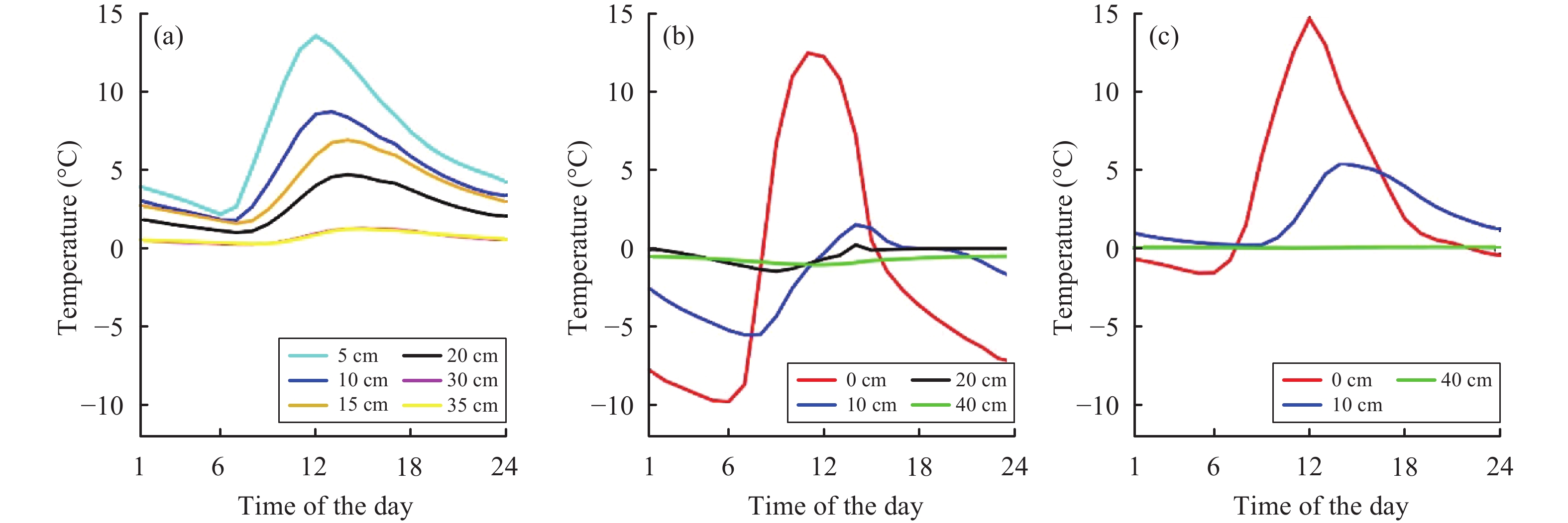
Figure 5 Mean daily cycles of debris temperatures at various layers of the debris on Lirung Glacier during 2013 (a) monsoon, and (b) winter, and 2014 (c) pre-monsoon seasons. Temperature measurements from both sites, i.e., AWS site and above AWS site were plotted for the monsoon season and data from the AWS sites were plotted for the winter and pre-monsoon seasons
4.2. Vertical temperature gradients
Vertical temperature gradients were calculated based on measured debris temperatures at different debris thicknesses during each season. The daily linear gradient with depth in the monsoon (−20.81 °C/m in September to October, 2013), winter (4.05 °C/m in December, 2013), and pre-monsoon (−7.79 °C/m in April, 2014) are of different magnitude, indicating heat flux away from the ice in the winter and heat flux towards the ice in the monsoon and pre-monsoon seasons. The highest difference of temperature between the surface and various depths was observed at 12:00 PM and lowest at 06:00 AM (Figure 6) during each measurement season, which indicates that highest temperature gradient was at 12:00 PM and lowest at 06:00 AM. This also specifies that maximum energy transfers from the surface to debris/ice interface at 12:00 PM.
Figure 6

Figure 6 Averaged debris temperature profiles for different time of the day at the different debris thicknesses that was measured at 0.10, 0.20 and 0.30 m in the (a) monsoon season and at 0 m (surface), 0.10 and 0.40 m during the (b) winter and (c) pre-monsoon seasons
4.3. Thermal diffusivity and thermal conductivity
Thermal diffusivity (α) was estimated for the monsoon and winter seasons (Figure 7). We can clearly see a better fit during the monsoon season (Figure 7a) than the winter season (Figure 7b). Values near to best fitted line are part of the conductive process and values dispersed around the line are due to the non-conductive processes such as convective and latent heat exchange. We can say that the conductive process appears to be dominant during the monsoon season, while other processes were dominant during the winter season. The value of α was found higher in the monsoon season (20×10−7 m2/s) than in the winter season (2×10⁻⁷ m2/s). Thermal conductivity (ke) of the debris was estimated using the values of α for the monsoon and winter seasons. Following Nicholson and Benn (2013), 10% error on the bulk volumetric heat capacity was assumed to estimate ke. We found a very high value of ke in the monsoon season, i.e., 2.71 ± 0.27 W/(m·K) than the winter season, i.e., 0.27 ± 0.02 W/(m·K) at AWS site.
Figure 7

Figure 7 Scatter plots of the first derivative of hourly temperature with time (dT/dt) against the second derivative of hourly temperature with depth (d2T/dz2). The total debris thickness of debris was 0.38 m for the monsoon season and 0.40 m for the winter season at the AWS site. The time period for the assessment of the derivatives: September 24 to October 3 2013 for (a) monsoon, and December 1 to 4 2013 for (b) winter. The slope of the best fitting line gives an approximation of the thermal diffusivity
4.4. DDF
DDF was calculated based on ablation stakes and daily air temperature for the monsoon, winter, and pre-monsoon seasons spanning the years of 2013 and 2014. We estimated DDF for different debris thicknesses ranging from 0.03 m to 0.42 m (Figure 8). The DDFs were 4.64, 2.43 and 5.71 mm/(°C·d) at 0.05 m debris thickness in the monsoon, winter, and pre-monsoon seasons, respectively. Similarly, the values were 2.45, 0.40, and 2.15 mm/(°C·d) at 0.20 m in the monsoon, winter, and pre-monsoon seasons, respectively. Highest DDF was found at the black colored dirty ice during the pre-monsoon (14.33 mm/(°C·d)).
Figure 8
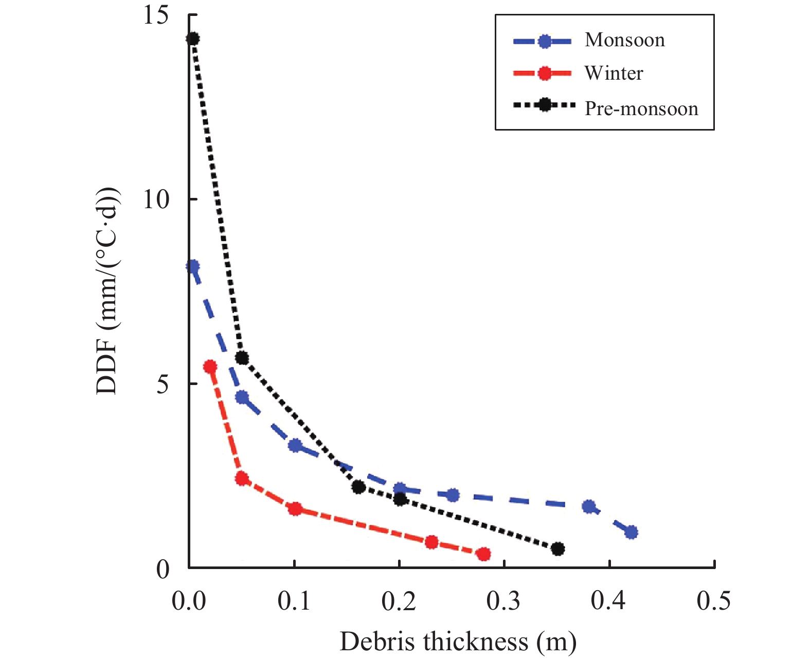
Figure 8 Degree-day factors for the monsoon, winter, and pre-monsoon seasons. The time period for the estimation of degree-day factor was from September 20 to October 3, 2013, November 30 to December 12, 2013, and from April 7 to 16, 2014 for the monsoon, winter, and pre-monsoon seasons, respectively
5. Discussion
Meteorological conditions and supraglacial debris properties could determine glacier ice melt in the debris-covered glaciers (Juen et al., 2013). Temperature measurements at different thicknesses including the surface of the debris are one of the widely used techniques to estimate thermal conductivity of debris overlying the ice. The three seasons spanning 2013 and 2014 show a marked difference in the behavior of the temperature profile. Temperature measurements in the monsoon season have a smaller range (maximum–minimum) compared to the winter and pre-monsoon seasons, which can be explained by frequent precipitation events in the form of rainfall during the monsoon season. This increases the moisture content in the debris, making it easier to transform the energy at higher depths and increases the temperature as well. Also, presence of cloud cover during most of the measurement period prevents the strong heating of the debris and reduces the temperature range. Temperature was decreasing downward with increasing lag time, with highest lag time in the winter season and least in the monsoon season. The decreasing trend of temperature was observed especially at the above AWS site as the winter proceeds from December 1 to 12 and low mean air temperature prevailed especially from the 4th of December (−0.33 °C) causing an inversion of the temperature gradient. The maximum surface temperature during the winter period rarely penetrated 0.2 m of debris during the measurement period which signifies that ice melt rarely occurs below this depth during this period. However, the diurnal temperature cycle penetrates about 0.3, 0.2, and 0.1 m deep during the monsoon, pre-monsoon, and winter seasons, respectively, which was also observed by Nicholson and Benn (2006).
We found different debris temperature profiles at different times of the day. However, the mean temperature measured at three different layers of the debris was approximately linear. It is obvious that temperature changes faster at the surface than at sub debris layers and leads to non-linear profiles, but it can be approximated by a linear gradient with 24-hour average temperatures (Nicholson and Benn, 2006). The linear gradient during the monsoon season was about three times the mean gradient over the pre-monsoon season, and the heat flux towards the ice is significantly higher in the monsoon period than in the pre-monsoon period. The lag time of the maximum temperatures between surface and subsurface layers was similar to the findings of Nicholson and Benn (2006); Reid and Brock (2014); Shahi et al. (2015), and varied by the time of day and season. The warming curvature of the temperature profiles at each time of day during the monsoon season suggests a transfer of heat towards the ice throughout the day.
Surface heat can transfer towards ice in the form of conduction, convection, radiation, advection, and phase changes. The values of α show significant differences between the monsoon and winter seasons. Seasonal variation in α is attributed to temperature-dependency of α, presence of liquid water and phase changes when the mean daily temperature is near 0 °C (Nicholson and Benn, 2013). They also discussed the influence of thermistor precision in estimation of α. In our case, the difference of temperature between 0.10 and 0.40 m was very low during the winter season. Therefore, using the methods of Conway and Rasmussen (2000) it is difficult to accurately estimate the value of α because the temperature sensors were unable to capture small changes in temperature accurately enough with depth and time. We estimated ke using the values of α, which is most suitable to estimate the sub-debris ablation in the debris-covered glacier and used by many scholars, e.g., Nicholson and Benn (2006); Reid and Brock (2010). Significant differences in ke have been found between monsoon and winter measurement periods. Higher value of ke in the monsoon season can be explained by the presence of water within the debris and consistent surface heating throughout the measurement period. The presence of water near the surface of the debris was from frequent rainfall events, and in the lower portion of the debris was from infiltration and ice melt during the monsoon season. Higher moisture content in the debris enables it to conduct heat more efficiently and increases the value of ke, which ultimately increases the melting of ice in the monsoon season than in the winter season. Presence of voids (Juen et al., 2013), grain size and the types of debris material also play a significant role in determining the value of ke. Reid and Brock (2010) noted a 10% increase in ice melt as they increased the value of ke by 10% in their model. They also mentioned the huge effect of the debris thickness and ke have on ice melt and debris properties. Knowledge of the lithology is required to determine ke, which is also suggested by Nicholson and Benn (2013). Study of the temporal and spatial variation of ke is largely dependent on debris properties and composition of the debris material that varies with time and spatially. Intensive study of the lithology, its distribution, and the debris thickness and arrangement from surface to debris/ice interface is required to understand ke of the debris. However, it is impractical for regional-scale studies, and remote sensing can be used to obtain information about debris thickness and thermal properties (Mihalcea et al., 2008; Foster et al., 2012; Schauwecker et al., 2015; Huang et al., 2017). Ground penetrating radar (McCarthy et al., 2017) is a useful tool for mapping debris thickness in the field to validate remote sensing results.
DDF can be easily calculated using ablation data from field measurements, e.g., Braithwaite (1995), Kayastha et al. (2000), Singh et al. (2000) and Xu et al. (2017). The values of DDFs are a result of ice melt and air temperature, and therefore varies with debris thickness and different glaciers (Kayastha et al., 2000). Solar radiation heat has a significant role in determining DDF in clean ice and snow. However, this is not the case for debris-covered glaciers because they are controlled by the energy available at the surface and heat conductivity in the debris. We found that DDF decreases with increasing debris thickness. Cumulative positive degree-days corresponding to each season was the same for different stake measurement sites and hence calculated DDF increases as melting increases. Therefore, DDF was highest at 0.003 m debris thickness, with a decreasing trend with the increase of debris thickness in each season. The highest value of DDF (14.33 mm/(°C·d)) at dirty ice was observed in the pre-monsoon season. This can be attributed to less positive degree days (Braithwaite, 1995) during the pre-monsoon season compared to the monsoon season, despite highest melting in the monsoon. Thermal conductivity of the debris played an important role in ice melt at higher debris thickness especially during the monsoon period. We obtained a higher value of ke (2.71 ± 0.27 W/(m·K)) in the monsoon season at 0.38 m and is responsible for higher DDF at higher debris thickness. This can be further described by thermal resistance (Kayastha et al., 2000), which decreases with the increase of debris thickness. The smallest values were found in the winter season at each measurement site compared to monsoon and pre-monsoon seasons, clearly a result of small ice melt during the winter period due to less conductive debris (ke = 0.27 ± 0.02 W/(m·K)). DDF for ice generally increases as altitude increases as explained by Kayastha et al. (2003) in Yala Glacier and Glacier AX010. However, in our case we could not point out the effect of increasing altitude. This is mainly due to three main reasons: (1) we used the same air temperature for all altitudes, (2) the altitude difference between stake measurements was less than 200 m, and (3) our stake measurement data were not at the same debris thickness at different altitudes. DDF is largely dependent on air temperature which can be a function of surface temperature rather than elevation in case of debris-covered glaciers (Foster et al., 2012; Steiner and Pellicciotti, 2016). However, surface temperature may vary when debris thickness changes significantly and changes the air temperature accordingly. This can be partly achieved by using several stake measurements at different altitudes at same thickness of the debris with air temperature measurement which is challenging in terms of heterogeneous surface of debris of different thermal properties, instrumentation, remoteness and cost.
6. Conclusion
This study presents the results of thermal diffusivity and thermal conductivity from debris temperature measurements, which are important characteristics of the debris material that have a significant role in debris-covered glacier melt. We found a large difference in the values of diffusivity and conductivity between the monsoon and winter seasons. A large value in the monsoon than in the winter season is attributed to large surface temperatures and more moisture content in the debris. Inversion of the mean temperature for longer duration in the winter season indicates the transfer of heat towards the surface, which helps the debris freeze as well. Understanding the relation of air temperature with ice melt at different thickness is helpful for estimation of ice melt using only air temperature when field measurements are lacking. The calculated values of ke and DDF would be useful in mass balance modeling, and glacio-hydrological modeling in a basin with debris-covered glaciers. However, field-based measurements, e.g., ice melt at same debris thickness at different elevations, and debris temperature measurements for all seasons are needed to aid in more accurate modeling. Such modeling efforts could estimate the surface lowering rates of the glacier and melt water availability in different seasons.
Acknowledgments:
We are very grateful to the HKH Cryosphere Monitoring Project implemented by the International Centre for Integrated Mountain Development (ICIMOD) and supported by the Norwegian Ministry of Foreign Affairs. We also like to thank the project partners for their help in carrying out this study, including the Himalayan Cryosphere, Climate and Disaster Research Center, Kathmandu University; Central Department of Hydrology and Meteorology, Tribhuvan University; Department of Hydrology and Meteorology, Government of Nepal; and Water and Energy Commission Secretariat, Government of Nepal; and Department of National Park and Wildlife Conservation, Government of Nepal. We would like to express thanks to Achut Parajuli, Rakesh Kayastha and Roshan Dahal for their assistance in field work. We express our gratitude to Himal Venture Treks and Exp. P. Ltd., Kathmandu and local people of Langtang Valley for the logistic support during field work.
Reference
Response of debris-covered glaciers in the Mount Everest region to recent warming, and implications for outburst flood hazards
DOI:10.1016/j.earscirev.2012.03.008 [Cited within: 1]
Planimetric and volumetric glacier changes in the Khumbu Himal, Nepal, since 1962 using Corona, Landsat TM and ASTER data
DOI:10.3189/002214308786570782 [Cited within: 1]
Multi-decadal mass loss of glaciers in the Everest area (Nepal Himalaya) derived from stereo imagery
DOI:10.5194/tc-5-349-2011 [Cited within: 1]
The state and fate of Himalayan glaciers
DOI:10.1126/science.1215828 [Cited within: 1]
Positive degree-day factors for ablation on the Greenland ice sheet studied by energy-balance modelling
DOI:10.1017/S0022143000017846 [Cited within: 2]
Glacial lakes of the Hinku and Hongu valleys, Makalu Barun National Park and Buffer Zone, Nepal
DOI:10.1007/s11069-013-0689-8 [Cited within: 1]
Seasonal variation of ice melting on varying layers of debris of Lirung Glacier, Langtang Valley, Nepal
DOI:10.5194/piahs-368-21-2015 [Cited within: 1]
A physically based method for estimating supraglacial debris thickness from thermal band remote-sensing data
DOI:10.3189/2012JoG11J194 [Cited within: 2]
Statistical analyses of the forms of the glaciers in the Khumbu himal
DOI:10.5331/seppyo.39.Special_7 [Cited within: 1]
Field experiment on glacier ablation under a layer of debris cover
DOI:10.5331/seppyo.39.Special_20 [Cited within: 1]
Contrasted evolution of glacial lakes along the Hindu Kush Himalaya mountain range between 1990 and 2009
DOI:10.1016/j.gloplacha.2010.10.003 [Cited within: 1]
A short-term field experiment on sub-debris melt at the highly maritime Franz Josef Glacier, Southern Alps, New Zealand
A simple model to estimate ice ablation under a thick debris layer
DOI:10.3189/172756506781828395 [Cited within: 1]
Estimation of supraglacial debris thickness using a novel target decomposition on L-band polarimetric SAR images in the Tianshan Mountains
DOI:10.1002/2016JF004102 [Cited within: 1]
Thermal properties of a supraglacial debris layer with respect to lithology and grain size
DOI:10.1111/geoa.12011 [Cited within: 6]
Contrasting patterns of early twenty-first-century glacier mass change in the Himalayas
DOI:10.1038/nature11324 [Cited within: 1]
Positive degree-day factors for ice ablation on four glaciers in the Nepalese Himalayas and Qinghai-Tibetan Plateau
Impact of a global temperature rise of 1.5 degrees Celsius on Asia's glaciers
DOI:10.1038/nature23878 [Cited within: 1]
Ground-penetrating radar measurements of debris thickness on Lirung Glacier, Nepal
DOI:10.1017/jog.2017.18 [Cited within: 1]
Spatial distribution of debris thickness and melting from remote-sensing and meteorological data, at debris-covered Baltoro glacier, Karakoram, Pakistan
DOI:10.3189/172756408784700680 [Cited within: 1]
Estimate of glacier ablation under a debris layer from surface temperature and meteorological variables
DOI:10.3189/s002214300001176X [Cited within: 1]
Estimate of ablation rate of glacier ice under a supraglacial debris layer
DOI:10.1111/geoa.1999.81.issue-4 [Cited within: 1]
Calculating ice melt beneath a debris layer using meteorological data
DOI:10.3189/172756506781828584 [Cited within: 5]
Properties of natural supraglacial debris in relation to modelling sub-debris ice ablation
DOI:10.1002/esp.3299 [Cited within: 6]
Ice melting under a thin layer of moraine, and the existence of ice cores in moraine ridges
DOI:10.1080/20014422.1959.11907953 [Cited within: 2]
Distribution and interannual variability of supraglacial lakes on debris-covered glaciers in the Khan Tengri-Tumor Mountains, Central Asia
DOI:10.1088/1748-9326/10/1/014014 [Cited within: 1]
An energy-balance model for debris-covered glaciers including heat conduction through the debris layer
DOI:10.3189/002214310794457218 [Cited within: 3]
Assessing ice-cliff backwasting and its contribution to total ablation of debris-covered Miage glacier, Mont Blanc massif, Italy
DOI:10.3189/2014JoG13J045 [Cited within: 1]
Effects of debris on ice-surface melting rates: an experimental study
DOI:10.3189/002214310792447725 [Cited within: 2]
Debris thickness of glaciers in the Everest area (Nepal Himalaya) derived from satellite imagery using a nonlinear energy balance model
DOI:10.5194/tc-8-1317-2014 [Cited within: 1]
Debris-covered glacier energy balance model for Imja-Lhotse Shar glacier in the Everest region of Nepal
DOI:10.5194/tc-9-2295-2015 [Cited within: 1]
Remotely sensed debris thickness mapping of Bara Shigri Glacier, Indian Himalaya
DOI:10.3189/2015JoG14J102 [Cited within: 1]
Spatially variable response of Himalayan glaciers to climate change affected by debris cover
DOI:10.1038/ngeo1068 [Cited within: 1]
Influence of a debris layer on the melting of ice on Lirung Glacier, Langtang Valley, Rasuwa, Nepal
DOI:10.3126/jhm.v9i1.15585 [Cited within: 2]
Degree-day factors for snow and ice for Dokriani Glacier, Garhwal Himalayas
DOI:10.1016/S0022-1694(00)00249-3 [Cited within: 1]
Variability of air temperature over a debris-covered glacier in the Nepalese Himalaya
DOI:10.3189/2016AoG71A066 [Cited within: 1]
The temporal and spatial variation of positive degree-day factors on the Koxkar Glacier over the south slope of the Tianshan Mountains, China, from 2005 to 2010
