1 Introduction

Snow cover has heat preservation effect on the covered ground (Zhang et al., 2008 ). Shanley and Chalmers (1999) demonstrated that soil frost penetration depth varies greatly from year to year and correlated negatively with snow depth. Fortier et al. (2011) discovered that thick road embankment acts as a snow fence favoring snow accumulation on embankment shoulders and toes, which insulates the ground surface, decreasing heat loss in winter, and prevents further ground freezing. Therefore, snow cover on roads is detrimental to embankment stability in permafrost regions (Figure 1a). There are several techniques to mitigate thaw settlement of permafrost embankments (Lai et al., 2014 ). One of the most widely used techniques is thermosyphon, including the application of pile and building foundations. Thermosyphons can remove heat near the evaporator section by the circulation flow of working fluid filled in the closed pipes (Lai et al., 2009 ). Thermosyphons were successfully used in the Trans-Alaska Pipeline System as early as 1970s (Heuer, 1979). Two-phase thermosyphons with improved productivity have been developed for soil cooling and freezing by Bayasan et al. (2008) . Usage of thermosyphons is advisable for fast soil freezing and cooling. Zhang et al. (2011) and Song et al. (2013) proved that thermosyphons have a significant effect on cooling down the underlying permafrost. Based on monitored data, Yu et al. (2016) analyzed cooling scope and period of two-phase closed thermosyphons and found that the cooling depth of thermosyphons reached to 12 m during the monitoring period and the cooling period was eight months at 2 m depth, which was one month longer than that at 4, 6, and 8 m depth, respectively. Dong et al. (2009) and Lai et al. (2009) analyzed the cooling effect of L-shaped thermosyphon embankment, and found that the structure has a good cooling effect on the embankment. Wu et al. (2014) proposed a thermal budget evaluation method to quantitatively analyze the cooling effect of thermosyphon embankment, and revealed that the annual average energy of the thermosyphons transferred in a year was 1,500 MJ to 2,000 MJ.

Previous studies on the application of thermosyphons in permafrost embankments were carried out in the snowless area of the Tibet Plateau. However, the application of thermosyphon embankment in snowy areas is seldom discussed. In this work, a numerical method is adopted to predict the thermal regimes of thermosyphon embankment based on the boundary conditions observed in snowy Northeast China. The results can be a reference for the application of thermosyphon embankment in snowy permafrost regions.

2 Method 2.1 Physical models and parameters

In order to investigate the effect of thermosyphon embankment, two physical models are considered. Case 1 only considers snow cover. In this situation, slopes, shoulders and the isolation strips of the embankment are covered by snow during the cold season. Geometrical sizes and strata of the model are determined according to Mobei Highway, Northeast China (Figure 2).

In accordance with drilling data, the soil is divided into four layers. From top to bottom is peat layer with plant roots, clay, gravel and bed rock, respectively. The height of embankment is 2 m. The slope gradient is 1:1.5. The thickness of the asphalt pavement is 18 cm. The road shoulder and the isolation strip are both 1 m wide. Each stratum is assumed to be uniform and isotropic. Due to symmetry of the model, a quarter of the model is extracted for computation in order to simplify the process. The thickness of the model is 2 m.

Case 2 is based on Case 1, by inserting thermosyphons at a 70° angle to the toe of the embankment. The evaporator section is 6 m long and the adiabatic and condenser section is 3 m long (Figure 3).

For numerical calculation, three-dimensional embankment models in two cases are both partitioned into 4-node tetrahedron elements by Comsol native function. Each element has four triangles. The maximum size of the grid is 1.5 m, and the minimum size is 0.008 m. The model in case 1 is partitioned into 54,566 units, and the model in case 2 is partitioned into 994,909 units. The simulated time span is 20 years, and the time interval for calculation is three days.

All soil types and physical parameters in the numerical simulations are listed in Table 1.

2.2 The governing differential equations and finite element method

In the computation of embankment temperature field in permafrost regions, apparent heat capacity method is applied. Ignoring heat convection and other heat effects, considering heat conduction and ice-water phase change only, and regarding unfrozen water content as the function of temperature, the temperature field of soil can be described with 3D-differential equation (Bonacina et al., 1973 ).

${C^*}\frac{{\partial T}}{{\partial t}} = \frac{\partial }{{\partial x}}\left( {{\lambda ^*}\frac{{\partial T}}{{\partial x}}} \right) + \frac{\partial }{{\partial y}}\left( {{\lambda ^*}\frac{{\partial T}}{{\partial y}}} \right) + \frac{\partial }{{\partial \textit {z}}}\left( {{\lambda ^*}\frac{{\partial T}}{{\partial {\textit {z}}}}} \right)$

(1)

At the moving boundary s(t), the continuity condition and the conservation of energy should hold, i.e.,

${T_{\rm f}}\left( {s\left( t \right),t} \right) = {T_{\rm u}}\left( {s\left( t \right),t} \right) = {T_m}$

(2)

${\lambda _{\rm f}}\frac{{\partial {T_{\rm{f}}}}}{{\partial n}} - {\lambda _{\rm u}}\frac{{\partial {T_{\rm{u}}}}}{{\partial n}} = L\frac{{{\rm d}s\left( t \right)}}{{{\rm d}t}}$

(3)

where f and u denote frozen and unfrozen states, respectively, L is latent heat of water (J/m³), T_m is the temperature on the freeze-thaw interface (°C), and n is direction vector of the moving boundary s(t) (m).

The fixed boundary is as follows:

$T = {T_a},\; - \lambda \frac{{\partial T}}{{\partial {n_1}}} = \alpha \left( {T - {T_a}} \right)$

(4)

Here, T₀ is the environmental temperature (°C), n₁ is the normal direction at the fixed boundary (m), and α is the coefficient of heat convection W/(m·°C).

The initial conditions are given as:

${T_{\rm u}}\left| {_{t = 0}} \right. = {T_0},\;{\Omega _{\rm u}}\left| {_{t = 0}} \right. = 0$

(5)

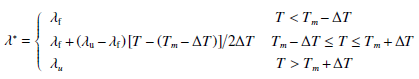
The apparent capacity method is adopted to determine the equivalent heat capacity in the phase change range (Lai et al., 2003 ).

${C^*} = \left\{ {\begin{array}{*{20}{l}}{{C_{\rm f}}}&{T < {T_m} - \Delta T}\\[6pt]{l/2\Delta T + \left( {{C_{\rm f}} + {C_{\rm u}}} \right)/2}&{{T_m} - \Delta T \le T \le {T_m} + \Delta T}\\[6pt]{{C_{\rm u}}}&{T > {T_m} + \Delta T}\end{array}} \right.$

(6)

and

(7)

Due to phase change of soil, temperature-dependent specific heat and heat conductivity, the computed problem is strongly nonlinear and cannot be solved analytically. Thus, numerical methods should be applied. The Galerkin method is adopted in this paper (Lai et al., 2003 ).

2.3 Boundary conditions

Temperature boundary is determined according to field observation data in Mohe, Northeast China. Temperature probes (Hobo U-12) developed by Onset company are used to measure boundary temperature. Its measuring range is from −40 °C up to 125 °C, and the precision is 0.22 °C. The measuring frequency is one time per hour. In all monitored boundary locations, the probe is buried 5 cm deep into the earth. After being fitted (with Matlab), the data can be deduced into different boundary temperature. They are described as:

Asphalt pavement:

$y = 1.39 + 24.88 * \sin (2{\text{π}}t/8760{\rm{ - }}0.7{\text{π}})$

(8)

Slope and road shoulder (with snow cover):

$y = 1.90 + 17.56 * \sin (2{\text{π}}t/8760{\rm{ - }}0.7{\text{π}})$

(9)

Median:

$y = 0.29 + 19.24 * \sin (2{\text{π}}t/8760{\rm{ - }}0.7{\text{π}})$

(10)

Nature surface:

$y = 0.03 + 15.99 * \sin (2{\text{π}}t/8760{\rm{ - }}0.7{\text{π}})$

(11)

Air temperature:

$y = {\rm{ - }}4.37 + 23.42 * \sin (2{\text{π}}t/8760{\rm{ - }}0.7{\text{π}})$

(12)

Slope and road shoulder (without snow cover):

$y = - 2.90 + 21.10 * \sin (2{\text{π}}t/8760 + {\text{π}}/2)$

(13)

The software computed the difference between air temperature and soil temperature around the thermosyphons. When the difference is equal to or greater than 0.8 °C, the thermosyphons start working, otherwise they stop working. Furthermore, the condenser section's effective heat dissipating area is 4.53 m², efficiency of fin is 0.8; convective heat transfer coefficient between air and condenser section can be described as (Sheng et al., 2006 ):

$\alpha = \left\{ \begin{array}{l}30 \,\, {\rm{W/}}({{\rm{m}}^{\rm{2}}} \cdot\! {\text{°C}}),\;\;\;\;\;\;{T_a} - T \ge 0.8,\\[6pt]0,\;\;\;\qquad \qquad \qquad {T_a} - T < 0.8.\end{array} \right.$

(14)

Heat transfer of thermosyphons is:

$Q = \alpha F\Delta T(t)$

(15)

Here, Q is heat transfer of thermosyphons; F is effective heat exchange area of thermosyphons; ΔT(t) is difference value between soil temperature around thermosyphons and air temperature. Because the thermosyphon has a thermal conductivity capacity several orders higher than that of the soils, the thermal resistor of the thermosyphon is not taken into account during the computation process. Thus, all heat Q of the thermosyphons is put on evaporation part as a linear heat flux (Zhuang and Zhang, 2000).

The bottom boundary of the model can be treated as heat flux. According to drilling data, the heat flux is 0.051 W/m at the depth of 70 m. The other boundaries are assumed adiabatic.

The observed data on September 28, 2011 in Mohe is applied as the initial temperature, which is presented in Figure 4. The simulated time span is 20 years.

3 Results and analyses

Permafrost in Northeast China usually reaches the maximum thawed depth around October 15 in a normal year. Figure 5 shows the temperature distribution of Case 1 on October 15 after 20 years of operation. As can be seen from the figure, the permafrost table under embankment center is −3.8 m. The permafrost table under nature surface is −4.9 m, which is lower than that under embankment center. The difference is mainly caused by embankment height, which raises the permafrost table (Zhang, 2004). Moreover, the permafrost table under slope toe is −5.4 m, which is 1.6 m lower than that under snowless embankment center. Figure 6 is the time-history curve of temperature at a depth of −5 m located in slope toe perpendicular line and center perpendicular line of embankment. As presented in the graph, positive cumulative temperature at −5 m slope toe line with snow is higher than that at −5 m center line of embankment without snow. The aforementioned results show that snow has heat preservation effect on permafrost, which can prominently affect permafrost environment under the snow, and accelerate permafrost degradation. The effect will increase potential security risk of roads, and certain measures should be taken to weaken heat preservation effect of snow.

Permafrost in Northeast China usually reaches the maximum frozen depth around April 15. In order to study the effect of thermosyphons on permafrost, the temperature field between common embankment (Case 1) and thermosyphon embankment (Case 2) at April 15 and October 15 in the 20 year were compared in Figure 7.

As presented in Figure 7a, embankments freeze completely, and temperature of both embankments can reach as low as −11 °C. The depth of −2 °C isotherm under slope toe of thermosyphon embankment (Case 2) is −10.7 m, which is 9.8 m higher than −20.5 m of −2 °C isotherm in common embankment (Case 1). This indicates that cooling effect of thermosyphon embankment is better than that of common embankment in cold seasons. After April 15, as the air temperature gradually increases, surface soil starts warming and melting. This procedure lasted until October 15 in the same year, when the thawed depth reaches maximum. Figure 7b is temperature filed between two kinds of embankment on October 15 in the same year. At this moment, permafrost table under slope toe of common embankment is −5.4 m, which is 1.23 m lower than −4.17 m of in thermosyphon embankment. It can be seen that the permafrost table at the centerline of Case 2 is little higher than that of Case 1. The ground temperature at the center area of Case 2 is colder than that of Case 1. It also can be seen that the effect area of thermosyphons is mainly at the slope foot of the embankment.

Figure8a is the time-history curve of temperature at the depth of −5 m under slope toe of two embankments. The depth of −5 m is in a shallow stratum, belong to permafrost active layer, thus the temperature fluctuates greatly with time. In accordance with Figure 8a, soil temperature with thermosyphon is always lower than that without thermosyphon at any given time. Figure 8b is the time-history curve of permafrost table under two kinds of embankment slope toe. As presented in Figure 8b, permafrost table of thermosyphon embankment under slope toe is always higher than that of common embankment at any year. Permafrost table of thermosyphon embankment under slope toe is 0.7 m higher than that of common embankment at the first year. As time progresses, the difference enlarges year by year. The permafrost table of thermosyphon embankment under slope toe is already 1.2 m higher than that of common embankment in the 20th year.

The aforementioned results indicate that thermosyphons help raise permafrost table under snow covered embankment slope, and greatly weaken heat preservation effect of snow. Overall, although slope toe is installed with thermosyphons, the permafrost table still slowly declines with time. The permafrost table of thermosyphon embankment under slope toe descends 0.26 m in 20 years, which indicate that thermosyphons alone cannot protect permafrost from degenerating.

4 Conclusions

At present, effect of snow cover on embankments in a snowy permafrost zone and its targeted mitigation technologies are rarely studied. This paper focuses on this issue based on real boundary conditions and initial ground temperature obtained in Mohe area, a snowy permafrost area in Northeast China. The common numerical methods used for thermal regime prediction of embankment in permafrost regions are adopted in this study. By analyzing the numerical simulations yield the following conclusions:

(1) During the simulated time span, the difference of thermal regimes between non-thermosyphons affected by snow cover and the embankment cooled by thermosyphons reaches to 22 m in depth below the ground surface. It is much warmer in the non-thermosyphon embankment body in winter. Affected by the snow cover, as time goes by, heat flux gradually spread into the deep ground of the subgrade, which could causes potential thaw settlement of the embankment.

(2) The permafrost table of the thermosyphon embankment is always higher than that of the non-thermosyphon embankment in each year. The permafrost table under the slope toe of thermosyphon embankment is 1.2 m higher than that of the non-thermosyphon embankment in the 20th year. In addition, the permafrost table at the slope toe of thermosyphon embankment goes deeper, 26 cm over 20 years. These results indicate that thermosyphons can greatly weaken the warm effect of snow cover, but it cannot avoid the degradation of permafrost under the scenarios of snow cover. Therefore, composite measures need to be adopted to keep embankment stability in snowy permafrost zones.

Acknowledgments:

This study was supported by the National Natural Science Fund (41571070), the Fund of SKLFS (SKLFSE-ZT-21), the Fund of the National Key Basic Research and Development Program (2012CB026102), the Funds of Key Research Program of Frontier Sciences of CAS (QYZDYSSW-DQC015) and fund HHS-TSS-STS-1502.