1 Introduction

The high altitude Hindu-Kush Karakoram and Himalaya (HKKH) range is a very important region in terms of its cryospheric resources, which provides melt water from snow and ice to several Asian watersheds such as the Ganges, Indus and Brahmaputra (Messerli et al., 2004; Panday et al., 2014 ). This snow and ice is the primary source of water for the major river basins of HKKH, and is important in agriculture, power production and domestic use for mountainous populations of HKKH. The amount of snow and ice in HKKH is surpassed only by the Polar Regions, which is why HKKH is considered as the third pole of our planet (Smiraglia et al., 2007 ). The economies of South Asia rely heavily on agriculture, which depends on the availability of water from HKKH (Akhtar et al., 2008 ). Thus, the current state of glaciers and their response to climate change in terms of future water availability will have important ramifications for south Asia. Reduction of ice mass may initially produce more melt water but eventually the amount of melt water will decline. On the other hand advancing ice masses can store more precipitation lead to reduce total runoff and may produce local hazards. Shigar River Basin lies with in Central Karakoram National park and covers most of the park area. Recent studies conducted in Central Karakoram National Park (CKNP) shows no significant change in glacier area i.e., +27 km² (Minora et al., 2013 ). Recent glacier status of Central Karakoram National Park also shows no remarkable area change (+0.6% from 2001 to 2010); (Bocchiola et al., 2013). For the Shigar River Basin, few glacio-hydrological studies have been conducted. Thus, our current study is important in acquiring information about future hydrological conditions under different representative concentration pathways RCPs climate scenarios for this basin. The present paper may also be of value to ongoing discussions regarding present and future water resource management. Shigar River Basin is a sub-tributary of the Upper Indus Basin, Central Karakoram, where snow and ice contributes more than 50% of water to the Indus River, Pakistan (Immerzeel et al., 2010 ). Total annual precipitation in central Karakoram range between 200 to 500 mm, although these values are derived from valley based meteorological stations and may not reflect higher elevation annual precipitation (Archer, 2003). However, measurements from accumulation pits above 4,000 m a.s.l. show 1,000 mm/a to more than 3,000 mm/a depending on the site (Winiger et al., 2005 ). In contrast, central Himalayas' (Nepal) receive about 80% of precipitation from summer monsoons in late summer (July~September) while during the winter season (December~February) displays very low flow that has large impact in availability of water (Adhakari, 2013).

Various studies have noted that Karakoram glaciers behave differently from glaciers in the Himalaya's, Europe and North America (Mayewski et al., 1979; Kick, 1989). Climatic conditions of central Karakoram is set in such a way that summer monsoons contributes very little in terms of precipitation, while during the winter season "westerlies" contributes in a major way to the accumulation of snow and ice. Also, the region of central Karakoram is classified as dry cold desert which is influenced by geological and geographic conditions (Bocchiola et al., 2011 ). Climatic, geological and geographical conditions seem to mitigate the effect of climate change in terms of glacier coverage in regions such as CKNP but not in central Himalaya, Nepal.

2 Study area

Shigar River Basin is located in Baltistan, northern Pakistan, nested within the upper Indus Basin, Central Karakoram, ranging from 35.28°N to 37.80°N latitude and 74.58°E to 76.58°E longitude, covering an area of 6,921.46 km² of which 2,813 km² (40%) is glaciated (Figure 1). About 80% of the total glaciated area contains clean ice and the remaining 20% is covered by debris. The basin starts from Shigar Bridge at 2,204 m a.s.l., maximum elevation of 8,611 m a.s.l. at Mt. K2, and about 45% of the basin lies above 5,000 m a.s.l. (Figure 2). Average altitude of the whole basin is 4,613 m a.s.l.. The Shigar River Basin is a sub-basin of Upper Indus Basin and snow and ice melt majorly contributes in discharge (Immerzeel et al., 2010 ). Climatic conditions in central Karakoram are influenced by westerlies in the form of winter precipitation of snow and ice, and very little for summer monsoons in the form of precipitation. According to KÖppen's climate classification, Shigar River Basin lies in a "cold desert" which implies very little precipitation and large variation in daily temperature ranges. The Nanga Parbat-Haramosh massif acts as a barrier to northward movement of monsoon storms, thus very few enter Central Karakoram of Pakistan (Bocchiola et al., 2011 ). Great uncertainty in precipitation at higher elevations has been found because meteorological data are derived from lower elevation meteorological stations.

3 Input data 3.1 Meteorological data

Meteorological data from Shigar River Basin and Skardu Station was collected from the Water and Power Development Authority of Pakistan (WAPDA) and Pakistan Meteorological Department (PMD), respectively. Shigar Automatic Weather Station (AWS) is located within the basin at an elevation of 2,369 m a.s.l. and Skardu AWS is located in Skardu about 15 km away from the basin boundary. Daily values of temperature and precipitation for the period of 1988 to 2015 were obtained from Skardu AWS, while data from Shigar AWS is available only for the period of 1996 to 2006 with significant missing data periods. Daily discharge from hydrometric station of WAPDA at Shigar Bridge is obtained from 1988 to 1997. Details of meteorological stations are presented in Table 1.

To simulate daily discharge from the entire Shigar River Basin we used daily precipitation and temperature values from Skardu AWS for the same overlapping period of available discharge information from Shigar hydrometric station from 1988 to 1997. Data from Shigar AWS was not continuous and complete. Therefore, we first correlated the available data from both Shigar and Skardu AWSs (r=0.86) and then used the meteorological data from Skardu AWS to tune our glacio-hydrological model for simulation of daily discharge. In current literature there is little knowledge of precipitation above 5,000 m a.s.l.. According to Young & Hewitt (1990), maximum precipitation in the Himalayan region took place at an elevation around 5,000 m a.s.l. and according to Immerzeel et al. (2015) , maximum precipitation of 1,271 mm/a was observed in the Upper Indus Basin at 3,750 to 4,250 m a.s.l. Immerzeel et al. (2012) used an inverse approach to estimate spatial distribution of precipitation in Hunza Basin by using glacier mass balance. Winiger et al. (2005) proposed a power law that may represent total annual precipitation for the Karakoram region up to 5,000 m a.s.l. Bocchiola et al. (2011) showed an increase in precipitation from 1,200 m a.s.l. to 3,000 m a.s.l., using the power law proposed by Winiger et al. (2005) . In present study we also use the power law proposed by Winiger et al. (2005) to extrapolate precipitation from ground station to higher elevations of up to 5,000 m a.s.l. (Equation (1)). Above this elevation we use a linear decreasing precipitation trend as presented in Equation (2) to the maximum elevation at Mt. K2 (8,611 m a.s.l.):

${P_y} = 9 \times {10^{ - 6}}\left({{{\textit {z}}^{2.22}}} \right)\;\;\;\;\;\textit {z} \le {\textit {z}_p} = 5000\;{\rm m}\;{\rm a.s.l.}$

(1)

$\begin{split}& {P_y} = 9 \times {10^{ - 6}}\left( {{\textit {z}^{2.22}}} \right) - \left( {\textit {z} - {\textit {z}_p}} \right)\frac{{9 \times {{10}^{ - 6}}\left( {{\textit {z}^{2.22}}} \right)}}{{{\textit {z}_l} - {\textit {z}_p}}}\\ & \textit {z} >{\textit {z}_p} = 5000\;{\rm m}\;{\rm a.s.l.}\end{split}$

(2)

where P_y is yearly amount of precipitation (mm) and z is the altitude (m a.s.l.), z_l is the maximum elevation of basin and z_p is 5,000 m a.s.l.. Power law proposed by (Winiger et al., 2005 ) is applied to Hunza and Shigar basins to estimate precipitation dependence on altitude and obtained results were reasonable (Bocchiola et al., 2011 ; Soncini et al., 2015 ).

3.2 Future climate data

In this study, future climate data from regional climate model (RCM) has been used. Outputs of daily temperature and precipitation values of Coordinate Regional Downscaling Experiment (CORDEX) for South Asia having a resolution of 50 km are extracted. CORDEX is an application of regional climate downscaling sponsored by World Climate Research Program to produce regional climate change scenarios. Here in this study two different (RCP4.5 and RCP8.5) climate scenarios are used. These climate scenarios are representative for greenhouse gas concentration trajectories after a possible range of radiative forcing values in 2100 relative to pre-industrial values of +4.5 W/m² and +8.5 W/m². Precipitation and temperature values are extracted for Shigar River Basin for the observe period 1985~1997 and for 2020 to 2099 by using R-studio software and are corrected by using Equations (3) and (4) for temperature and precipitation, respectively. Number of methods are introduced for bias-correction. Traditional model output statistics (ETAMOS) require a relatively long training period while the Kalman filter requires a relatively short training period (about 4~5 days). A statistical method proposed by Cheng and Steenburgh (2007) was found to be reliable and used for temperature correction (Equation (3)):

${T_{{\rm{corrected}}}} = \left({{{{T}}_{{\rm{mod}}}} - T{'_{{\rm{mod}}}}} \right)*\frac{{\sigma {{{T}}_{\rm {obs}}}}}{{\sigma {{{T}}_{\rm{mod}}}}} + {{T}}{{\rm{'}}_{\rm{obs}}}$

(3)

where T_corrected is corrected temperature, T_obs and T_mod are observed and modeled daily temperatures, respectively, $T{'_{{\rm{mod}}}}$ is mean daily modeled temperature and $T{'_{{\rm{obs}}}}$ is mean daily observed temperature. Data from General Circulation Models (GCMs) are known to have a bias in precipitation. However for bias correction of precipitation (P_corrected) we used the relation proposed by Sperna Weiland et al. (2010) as presented in Equation (4):

${P_{{\rm{corrected}}}} = {P_{\rm {mod}}}\frac{{{{\dot P}_{\rm {obs}}}}}{{{{\dot P}_{\rm {mod}}}}}$

(4)

where ${\dot P_{\rm {obs}}}$ and ${\dot P_{\rm {mod}}}$ are mean observed and modeled precipitation, respectively and P_mod represents daily modeled precipitation for the study period.

3.3 Glacier cover area

Two Landsat images of August 2009 of 30 m resolution with minimum cloud and snow cover have been used for extraction of glacier cover area of Shigar River Basin. Pre-processed void free Shuttle Radar Topography Mission (SRTM) Digital Elevation Model (DEM) of 90 meter resolution is used to delineate the Shigar River Basin watershed. The extracted information regarding topography, i.e., slope, aspect, hill shade and elevation of the basin are combined with Landsat images to obtain better results for supervised maximum likelihood classification of land features. To improve classification results, we combined all visible and infrared Bands of Landsat images (except thermal band) with surface layers which successfully masked out debris covered ice under thick clouds (Khan et al., 2015 ). Then a hypsograph is prepared which shows 8% of total basin area is covered by debris-covered ice, 38% covered by clean ice and the remaining covered by rock and vegetation as presented in Figure 2.

4 Methods 4.1 The Glacio-hydrological model

The present study used a semi-distributed glacio-hydrological model called the Modified Positive Degree Day Model (MPDDM) developed by the Himalayan Cryosphere, Climate and Disaster Research Center (HiCCDRC), Kathmandu University, Nepal. This model calculates snow and ice melt from clean glacier area and ice melt under a debris layer using a corresponding positive degree day factors. Surface runoff from these melts, rainfall and base flow will provide total discharge which is then subjected to losses and routed for final discharge. MPDDM assumes that the melting of snow or ice is proportional to the positive degree-days linked by positive degree day factor. This is a simplification of complex processes that are properly described by a surface energy balance equation (Braithwaite and Olesen, 1989). This approach is appropriate in regions with scarce data as it requires less input data and uses a simple equation to estimate melt (Kayastha et al., 2000 ; Hock, 2003). Hence, in the present study, the PDD model, as used by Kayastha et al. (2005) and Pradhananga et al. (2014) for the estimation of monthly snow and ice melt from the glacierized river basin has been modified to estimate daily snow and ice melt and daily discharge from this basin and also projects future basin discharges with relative contribution of the runoff components.

A flow chart for MPDDM is presented in Figure 3. The whole basin is divided into 26 altitude belts with equal intervals, each zone separated into three types of land features, i.e., clean ice, debris covered ice and rock and vegetation. Air temperature for each altitude belt is obtained by applying local lapse rate of 0.0075 °C/m (Mihalcea et al., 2006 ). Daily snow and ice melt and ice melt under a debris layer are calculated by using Equation (5):

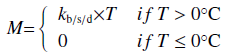
(5)

where Mis melt (mm/d), T is air temperature (°C) and k_b/s/d are positive degree day factor for bare ice, snow and debris covered ice melt (mm/(d·°C)). Degree day factors for snow and ice of low and high elevations are used separately, that is defined as the elevation up to 5,000 m a.s.l. is considered as low elevation while area of basin above 5,000 m a.s.l. is considered as high elevation. The model uses two monthly runoff coefficients C_r and C_s for rain and snow, respectively. Runoff coefficient expressing the losses as a ratio of measured precipitation to measured runoff, and two constant recession coefficients are obtained from recession flow plot (Martinec and Rango, 1986). These two coefficients represent the proportion of daily melt water which immediately appears in the runoff. There is a large scarcity of ground data in regard to altitudinal variation in the form of precipitation. Thus, it is very difficult to set a critical temperature to separate snow and rain. Snow is separated from rain by using critical temperature of 2 °C in such a way that the precipitation below the critical temperature will precipitate in the form of snow and precipitation at a higher temperature than critical value will be rain (Kayastha et al., 2000 ). For each time step snow and rain fall are separated as presented in Equation (6):

$\!\!\!\! \begin{array}{l}{\rm{Precipitation}} = {\rm{Snow}}\;\;\;\;\;\;\;\;\;\;\,\,\,\,\,\,\,\,\,\,\,\,\,\, if\;T \le 0\left({{\rm{All}}\;{\rm{Snow}}} \right)\\[7pt]{\rm{Precipitation}} = {\rm{Snow}} + {\rm{Rain}}\;\;\;\;if\;0 < T \le 2\left({{\rm{Snow}} + {\rm{Rain}}} \right)\\[7pt]{\rm{Precipitation}} = {\rm{Rain}}\;\;\;\;\;\;\;\;\;\;\;\;\;\,\,\,\,\,\,\,\,\,\, if\;T > 2\left({{\rm{All}}\;{\rm{Rain}}} \right)\end{array}$

(6)

Since the MPDD model cannot separate base flow itself, base flow separation is carried out in R-studio with the help of an inbuilt package 'EcoHydRology version 0.4.12' which has been used in a number of hydrological studies (Silwal et al., 2016 ). This is an automated method that uses a digital filter technique that associates high frequency waves with direct discharge, and low frequency waves with the base flow (Nathan and McMahon, 1990; Eckhardt, 2005). The digital filter generates higher base flow under peak flow conditions which corresponds to actual conditions.

The discharge in each altitude belt is calculated as a sum of runoff due to snow and ice melt, precipitation and base flow as given in Equation (7). Then the discharge from each zone is summed to provide discharge from the entire basin as given in Equation (8). The flow chart of MPDDM is presented in Figure 3.

${Q_{\textit{z} = }}{Q_{\rm r}} \times {C_{\rm r}} + {Q_{\rm s}} \times {C_{\rm s}} + {Q_{\rm b}}$

(7)

where Q_z is discharge (m³/s) from zone (z) and Q_r and Q_s are contribution of rain, ice and snow melt in discharge as mentioned in Martinec (1975) while Q_b is base flow (m³/s).

$Q = \mathop \sum \limits_{z = 1}^{z = n} {Q_z}$

(8)

Discharge is then routed to the basin outlet as per the recession equation (Equation (9)) given by Martinec (1975):

${Q_n} = Q \times \left({1 - K} \right) + {Q_{n - 1}} \times K$

(9)

where, Q_n is discharge (m³/s) on the n^th day and K is recession coefficient.

4.2 Accuracy assessment

Efficiency and performance of the hydrological model is generally represented by comparison of simulated and observed variables. Comparison between simulated and observed discharge are made at the catchment outlet. The Nash-Sutcliffe efficiency index (Nash and Sutcliffe, 1970) is used to assess the goodness of fit between simulated and observed discharge (Equation (10)). Volume difference is also used to determine model accuracy and increased confidence in the obtained simulated results.

$NS \! E = 1 - \frac{{\mathop \sum \nolimits_{i = 1}^n {{\left({{Q_i} - Q_i'} \right)}^2}}}{{\mathop \sum \nolimits_{i = 1}^n {{\left({{Q_i} - \bar Q} \right)}^2}}}$

(10)

where n is the number of days, Q_i is observed daily discharge, $Q_i'$ shows simulated daily discharge and average measured discharge of the given period is denoted by $\bar Q$ .

While volume difference is calculated by using the following relation as presented in Equation (11).

$VD = \frac{{{V_R} - V_R'}}{{{V_R}}} \times 100{\text{\%}} $

(11)

V_R Measured discharge and $V_R'$ shows simulated discharge.

The results for the accuracy assessment of remotely sensed data is presented in Table 4.

5 Results and discussions 5.1 Model calibration and validation

The model has been calibrated for the period of 1985 to 1992 while the period from 1993 to 1997 is taken as the validation period. After obtaining significant results from calibration, we tested the model for the validation period. We also performed cross-calibration and cross-validation. For this we simply changed the calibration period into validation and validation period into calibration and the obtained results were similar. Table 2 shows the parameters and values which are used for calibration. Among the input parameters, degree day factor for snow and ice seems to be most sensitive for changes in discharge. Degree day factors for snow 1~14 mm/(d·°C) are used (Singh et al., 2000 ) and zonal degree day factors for clean and debris covered ice are 1.13~7.78 mm/(d·°C) are used (Mihalcea et al., 2006 ).

Mean daily simulated discharge for calibration period from 1988 to 1992 and validation period 1993~1997 at catchment outlet are 219.07 m³/s and 221.79 m³/s against the observed values 221.05 m³/s and 238.09 m³/s, respectively. The Nash-Sutcliffe coefficient of 0.86 and volume difference of 0.9% were found during calibration period while for validation period, a Nash-Sutcliffe coefficient is 0.78 and volume difference is 6.85%. Model results are quite satisfactory for both calibration and validation periods against the observed values. By observing meteorological variables with discharge values obtained from ground stations during the study period 1988 to 1997, it shows peak flow during summer season when there is maximum temperature (Figure 4), while only 18% of the total precipitation from 1988 to 1997 took place during summer seasons. Figure 4 shows that precipitation is relatively very low in summer season whereas the contribution of snow and ice melt increases because of the higher temperature that leads to the melting of snow and ice.

Model simulated result for calibration period (1988 to 1992) shows good fit with observed values (Figure 5), while discharges are well represented during the low and peak flow, except for the year of 1988 and 1990. This might be due to uncertainties like glacial lake outburst flood and the uneven meteorological event at the higher elevation of the catchment like cloud burst. Precipitation is taken from the ground station that is established at lower elevation so it might not be well representative for higher elevations (Bocchiola et al., 2011 ; Immerzeel et al., 2015 ). In this study precipitation from the reference station are extrapolated by using power law proposed by Winiger et al. (2005) , and used the obtained precipitation values for calculation of gradient for each altitude belt, and compared our results with other studies (Immerzeel et al., 2015 ) and found similar results that the basin receives maximum precipitation around 3,500 to 5,000 m a.s.l. Variation of ground properties within the same altitude belt may also lead to reduce model efficiency, like MPDDM uses a single value k_b, k_d, and k_s for the whole altitude belt. The model is slightly over-estimating mean annual discharge during peak flow (August) and also during low flow period (October) as presented in Figure 5. Maximum discharge simulated by the model for calibration period is 823 m³/s and 733 m³/s during July and August, respectively whereas minimum flow of 29 m³/s is in January. While in validation period (1993~1997) discharges are slightly overestimating for the year of 1994, mean monthly discharge for validation period is represented quite well but few a peak flow events are not caught by the model (Figure 6). Maximum flow is simulated for July and August as 847 m³/s and 751 m³/s, respectively and minimum discharge for the month of March is 21 m³/s.

MPDDM can simulate daily discharge for poorly gauged basin with a good accuracy. MPDDM is considerably simple in view of complex dynamics of snow and ice melt including debris covered ice. Energy based glacio-hydrological models are also proposed (Nicholsona and Benn, 2006) but they may require more information. The model presented in the current study requires few input data like land cover information, degree day factor for snow, clean and debris covered ice and daily air temperature and precipitation.

5.2 Contribution of snow and ice melt in discharge

The mean annual contribution of snow and ice melt and rain and base flow for both calibration and validation periods are presented in Figures 7 and 8, respectively. During the calibration period, 32.37% of stream annual runoff is from snow and ice melt and the remaining 67.63% is contributed by rain and base flow. January, February and March contributes only 13.25% of stream mean annual flow, and precipitation contributes very little because of low temperature during these three months. During the same period the basin receives maximum precipitation because the lower temperature maximum precipitation should be in the form of snow. On the other hand, June, July and August display maximum discharge, where 89.21% of the annul flow take place (Figure 7). The relative annual contribution of rain and base flow reaches a maximum value of 58.48% and snow and ice melt contributes 30.73% of the stream flow during June, July and August. Minimum stream flow of only 12.90% of mean annual discharge is displayed during winter season (October to December).

For the validation period snow and ice melt contribution was 33.01% in discharge and the mean annual rain and base flow contributions were about 66.99% (Figure 8). Thus, simulated results for the study period (1988~1997) shows that the contribution of snow and ice melt varies with time that depends on the variation in temperature and amount of precipitation the basin receives. Snow and ice melt contribution is comparatively higher in the Shigar River Basin as compared to central Himalaya's. This difference might be due to the large glacier cover area in the Shigar River Basin as compared to those of Langtang and Sangda River basins (Pradhananga et al., 2014 ; Silwal et al., 2016 ), and the difference in precipitation and temperature values. In contrast, central Himalaya receives maximum precipitation during the monsoon season and Shigar River Basin receives maximum precipitation in the winter season.

5.3 Future hydrological conditions under different climate scenarios

For the estimation of future discharge two RCP scenarios have been adopted. Future climate data output from CCAM (CNRM) experiment of CORDEX is used having 50 km resolution. The Regional Climate Model (RCM) used for downscaling is CSIRO-CCAM and the driving GCM is CNRM-CM5. Extracted temperature and precipitation data from CORDEX-South Asia, for RCP4.5 and RCP8.5 climate scenarios are given as input to the model. Both scenarios show no significant trend of temperature, meanwhile the average annual temperature shows slightly higher values as compared to the observed period. In RCP8.5 precipitation shows slightly higher precipitation as compare to observed period of 1988 to 1997 with significant variation during 2045 to 2099. Precipitation in RCP4.5 and RCP8.5 increases by 17% and 73%, respectively from 2020~2099 as compared to observed period from 1988 to 1997. At the end of 21^st century temperature is higher in RCP8.5 as compared to that of RCP4.5 as presented in Figures 9 and 10. By analyzing future meteorological variables in both climate scenarios, RCP4.5 and RCP8.5 show similar conditions of higher precipitation in years 2028, 2029 and 2030. For example, 683, 1,928 and 1,127 mm, respectively in RCP4.5 and 605, 1,789 and 1,073 mm, respectively in RCP8.5. Temperature shows a different trend as compared to RCP4.5 climate scenarios from 2020 to 2099 but in 2028, 2029 and 2030 mean annual temperature also displays the similar kind of values in both scenarios. For example, 12 °C, 13 °C and 12 °C, respectively in RCP4.5 and 12 °C, 13 °C and 12 °C, respectively in RCP8.5.

In response to the projected meteorological variables RCP4.5 (Figure 9) shows slightly lower discharge throughout the whole period from 2020 to 2099 as compared to RCP8.5. In RCP4.5 discharge increases from 242 m³/s to 246 m³/s during the decades of 2020~2029 and 2050~2059, respectively (Figure 11). The discharge decreases at the end of decade 2090~2099 with a value of 199 m³/s. In RCP8.5 discharge is higher in 2020~2029 (260 m³/s) while mid-century 2050~2059 discharge is 220 m³/s but towards the end of the century it declines to 230 m³/s for the decade of 2090~2099 (Figure 12).

Both river discharge and temperature show a slightly increasing trend in RCP4.5 climate scenario. Average discharge for the entire period of 2020~2099 under the RCP4.5 scenario is 233 m³/s which is slightly higher than the observed average discharge of 229 m³/s for the study period. In contrast, RCP8.4 scenario shows a slightly decreasing trend in both temperature and discharge (Figures 10 and 12). Average mean annual discharge for RCP8.5 is 237 m³/s with some high flow peaks for 2017, 2033 and 2049 with mean annual discharge of 293, 285 and 275 m³/s, respectively. There are also low flows for years 2022, 2023, 2036 and 2037 with discharge of 232, 232, 160 and 237 m³/s, respectively. RCP4.5 displays a more variable flow regime as compared to our observed study period of 1988 to 1997.

While comparing the projected discharge (2020 to 2099) of both climate scenarios with observed discharge (1988 to 1997), average annual stream flow shows higher values then the study period discharge as presented in Table 3. RCP4.5 scenario shows higher discharge in all months except December to April which is because of the increasing summer temperature trend that intensifies glacier melt which leads to release of additional water. Mean summer temperature (June, July and August) is 23.7 °C for the period of 1988 to 1997 but increases to 23 °C for 2020 to 2099 in RCP4.5. RCP8.5 scenario shows a mean summer temperature of 22.5 °C which is almost equal to the observed period values.

5.4 Contribution of snow and ice in future projected discharge

Contribution of snow and ice melt in RCP4.5 scenario for the period 2020~2099 is about 36% while rain and base flow contributes about 64%. In RCP8.5 climate scenario snow and ice melt contribution is about 37% and rain and base flow contributes 63% in total discharge. Figures 13 and 14 represent the contribution of snow and ice melt for both RCP climate scenarios. Results for RCP4.5 scenario show that the snow and ice melt contribution extends to greater portion of the year (Figure 13) because of higher temperatures. Higher contribution of snow and ice melt during the months of May to October is mainly due to maximum air temperature during these months. RCP8.5 scenario also shows a similar trend for contribution of snow and ice melt from May to October because of increasing temperature (Figure 14). Snow and ice melt contribution varies significantly throughout the whole century on both RCP climate scenarios. RCP4.5 snow and ice contribution reaches maximum values during the period of 2020 to 2040 while declining at the end of the century. RCP8.5 shows slightly higher concentration of snow and ice melt contribution as compared to that of the RCP4.5.

In both RCP4.5 climate scenarios discharge is increasing in spring season because of increasing temperatures in winter and spring by +1.20 °C/a and +0.97 °C/a, respectively. Also, discharge shows a decreasing trend in summer and autumn of −0.71 °C/a and −1.47 °C/a, respectively. A similar kind of increasing discharge is simulated for the RCP8.5 climate scenario, in winter and spring temperature increases by +1.27 °C/a and +1 °C/a, respectively while during summer and autumn by −0.71°C/a and −1.47 °C/a, respectively.

5.5 Sensitivity analysis

Sensitivity analysis has been done by changing temperature, precipitation and glacier area. Temperature and precipitation increased and decreased by ±1 °C and ±2 °C and precipitation by ±10% and ±20%. Similarly, glacier area has been treated by ±5%, ±10% and ±15%. Temperature was found to be the most sensitive variable among these three. By increasing temperature by +1 °C and +2 °C discharge increased by 4.71% and 10.39%, respectively while decreasing temperature by −1 °C and −2 °C mean annual discharge decreased by 4.72% and 8.54%, respectively (Figure 15). Change in precipitation by ±10% and ±20% shows no significant change in discharge (Figure 16). Variation in precipitation does not affect discharge as much as temperature because maximum precipitation in the basin is during the winter in the form of snow which needs higher temperatures to melt. Changing glacier area shows slight changes in mean annual discharge of the basin (Figure 17).

6 Conclusion

Degree day approach for snow and ice melt is simple and computably fast enough for long term simulation, while soundly discerns the observed pattern of snow and ice melt. Average annual discharge simulated for the calibration and validation periods is 219 and 221 m³/s, respectively. MPDDM is sufficient to simulate daily discharge from the glaciated basin. Model simulated results reveal that snow and ice melt contributes significantly to total discharge. The Shigar River Basin shows maximum discharge during the summer season because of higher temperatures with maximum snow and ice melt contribution at the same time as compared to other seasons of the year.

Discharge likely increases in both projected climate scenarios due to increasing temperature and precipitation trend. Other studies conducted in the catchment also show possible consequences of warmer, wetter climate and increasing stream flow until the end of 21^st century. Contribution of snow and ice melt in total discharge increases up to 9% and 12% in both adopted climate scenarios of RCP4.5 and RCP8.5, respectively as compare to the observed period (1988~1997). This increase may be due to increasing temperature trend in both projected climate scenarios. Among the input variables temperature seems to be the most sensitive for hydrological response of the basin. Snow and ice contributes significantly to discharge in the Shigar River Basin. Contribution of snow and ice melt in total discharge depends on temperature, where changes in temperature can change the melt rate of snow and ice that ultimately affects river discharge. There are large uncertainties in future hydrological conditions of the glaciated catchment. However, hydrological response of the Shigar River Basin depends on meteorological conditions. Future increasing trend of temperature during winter and spring seasons in both adopted climate scenarios lead to reduced ice accumulation by changing the form of precipitation (snow into rain fall), earlier melt of fresh seasonal snow, and exposing the ice surface to melt. This may also lead to reduced ice volume. Possible increase in temperature may lead to increase discharge by increasing snow and ice melt contribution in total discharge. Accelerated ice melting will lead to increase in floods and hazards associated with the cryospheric environment. The current study describes a simple tool that can be used to assess future hydrological scenarios in a glaciated catchment, and can also be useful for management of water resources and adaptation purposes.

Acknowledgments:

This study is conducted under the auspices of Contribution to High Asia Runoff from Ice and Snow (CHARIS) and funded by United States Agency for International Development (USAID). For completion of this research work, in particular, we express our sincere thanks to CHARIS Project for their financial support and assistance in so many matters and the administration of Himalayan Cryosphere, Climate and Disaster Research Center, Kathmandu University. We also express our gratitude to the kind responses of Water and Power Development Authority of Pakistan (WAPDA) and Pakistan Meteorological department (PMD) for providing ground data. We express our sincere thanks to friends and fellows, for their kind advice and moral support.