Article Information
- YanLin Zhang, XiaoLi Chang, Ji Liang, DongLiang Luo, RuiXia He . 2016.
- The efficacy of Kriging spatial interpolation for filling temporal gaps in daily air temperature data: A case study in northeast China
- Sciences in Cold and Arid Regions, 8(5): 441-449
- http://dx.doi.org/10.3724/SP.J.1226.2016.00441
Article History
- Received: April 11, 2016
- Accepted: June 21, 2016
2. State Key Laboratory of Frozen Soils Engineering, Northwest Institute of Eco-Environment and Resources, Chinese Academy of Sciences, Lanzhou, Gansu 730000, China
Northeast China is the southernmost part of the Eurasian cryosphere, and it has the second largest expanse of permafrost (primarily in the form of latitudinal permafrost) in China (Wei et al., 2011; Luo et al., 2014b). Due to its thin and warm nature, the permafrost in this region is very sensitive to climate change and anthropogenic activities. According to the latest research, global warming has led to notable shrinkage in the permafrost areal extent in this region during the recent decades (Jin et al., 2007, 2010, 2011; Chang et al., 2013; Luo et al., 2014a; Beck et al., 2015; Bockheim, 2015; Sannel et al., 2016). This has received increasing attention from scientists, engineers, and governmental administrators. Extensive permafrost degradation may result in the release of a significant amount of CH4 and CO2 stored in organic frozen soils, and may lead to obvious changes in hydrological and ecological systems (Serreze et al., 2000; Christensen et al., 2004). Quality-controlled, serially complete climate datasets, especially daily air temperature, are very essential to evaluating and modelling the progresses and influences of climate change and its environmental consequences. The need for accurate daily climate datasets has never been greater. However, due to malfunctions and location changes of observing stations, temporal gaps (i.e., missing data) are common in the collected daily air temperature data, which reduces its utility. Gaps in daily air temperature data can even result in wrong monthly or annual means (Stooksbury et al., 1999). Therefore, before further data analysis and use, such gaps must be first identified and filled. Extreme errors in the data can also be removed and then filled in as missing data.
Numerous gap-filling approaches have been developed for estimating erroneous or missing data, including (1) methods based on temporal interpolation using information available within the daily series; (2) methods based on spatial information; and (3) methods based on both spatial and temporal information. Temporal interpolation estimates the missing value at a given time using values from different points in time, which is effective for short gaps, e.g., for one or a few steps of missing data (Kandasamy et al., 2012). Approaches using information from nearby data sources (stations) are necessary for filling long gaps. The simplest method is to estimate the missing data at a given time at a station to be a value or values from the nearest neighbor station or the mean of observed values at stations in the vicinity. The nearest-neighbor method is simple but prone to errors due to microclimate responses. Replacement by the mean or median misses extreme events and tends to artificially reduce spatial variation (Guttman, 1991).
Spatial interpolation is a potential method for filling temporal gaps at a given station through using information from surrounding (non-gap) stations; it includes the normal ratio method, inverse distance weighting, optimal interpolation, multiple regressions, and geostatistical methods (e.g., Kriging) (Rossi et al., 1994; Addink, 1999; Eischeid et al., 2000). Gap-filling methods based on both spatial and temporal interpolation have also been reported recently, but they are complex and time-consuming (Weiss et al., 2014).
Although Kriging methods have long been utilized for temporal gap-filling and spatial interpolation (Cressie, 1990), their accuracies and uncertainties should be assessed before further use and making decisions. Are there any temporal and spatial patterns in estimation uncertainties in a given region with a specific observation network? Such knowledge is still insufficient. The objective of this study was to assess the efficacy of Kriging spatial interpolation for filling the temporal gaps in daily air temperature data in northeast China. A cross-validation experiment was conducted and the temporal and spatial variations in estimation uncertainties were also checked, which are important for a wide variety of assessments and models needing daily air temperature data as inputs.
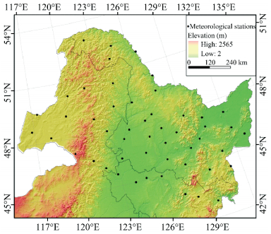
2 Materials and methods 2.1 Data collectionFifty stations from the national meteorological observation network were selected to fully cover the areal extent of the permafrost in northeast China, and their locations are shown in Figure 1. The daily mean (Tmean), maximum (Tmax), and minimum (Tmin) of air temperatures at these stations from January 1, 1960 to December 31, 2012 were used for analysis. The counts of the stations with different temporal gap length in days, i.e., the times of continuous missing data, are listed in Table 1. In the collected dataset, most temporal gaps of missing data last for only one or two days, and they can be easily estimated through temporal interpolation using temperatures from previous and post days. However, the temporal interpolation is not efficient for filling long gaps of continuous missing data (e.g., gaps lasting for over 10 days) (Kandasamy et al., 2012). In the dataset, there are about five stations with some temporal gaps of missing data lasting for months or even over a year.
|
| Figure 1 Meteorological stations in the study area |
| Type of missing data | Gap < 10 d | Gap 10~30 d | Gap > 30 d |
| Tmean | 18 | 1 | 4 |
| Tmax | 26 | 1 | 5 |
| Tmin | 36 | 2 | 5 |
Kriging spatial interpolation is often used to predict values of a variable at unmeasured locations with available measurements at neighboring sampled sites. It is an optimal, unbiased linear method with consideration of spatial correlation, and is often used for spatial data visualization, spatial query of properties, and spatial decision-making processes in geography, earth sciences, and environmental science (Cressie, 1990; Diggle and Ribeiro, 2007; Meng et al., 2013). Different methods were developed for univariates, such as simple Kriging, ordinary Kriging, and Kriging with a trend model (KT). The variants can be distinguished according to the treatment for local trend. In some literatures, KT is also referred as universal Kriging (UK) (Deutsch and Journel, 1998; Wackernagel, 2003). Some algorithms incorporating continuous or categorical auxiliary predictors have also been developed, such as blocking Kriging, co-Kriging, and Kriging with an external drift (KED) (Goovaerts, 1997). Actually, UK and KED are basically the same technique. The difference is that only coordinates are used as auxiliary predictors in KT, e.g., x and y in a two-dimensional space, while auxiliary variables other than coordinates are used in KED (Hengl, 2007). In the case of UK or KED, predictions at new locations are described as follows:
| ${Z^*}({{\bf{u}}_{\bf{0}}}) = \sum\limits_{i = 1}^n {{\omega _i}({{\bf{u}}_0}) \cdot Z({{\bf{u}}_i})} $ | (1) |
| $\sum\limits_{i = 1}^n {{\omega _i}({{\bf{u}}_0}) \cdot {f_k}({{\bf{u}}_i})} = {f_k}({{\bf{u}}_0})\;\;\;k = 0, 1, \cdots, p$ | (2) |
| $\sum\limits_{i = 1}^n {{\omega _i}({{\bf{u}}_{\bf{0}}}){\rm{ = }}1} $ | (3) |
where Z is the variable to be interpolated, Z
| ${\omega _0} = {\left\{ {{\omega _1}({{\bf{u}}_0}), \cdots, {\omega _n}({{\bf{u}}_0}), {\psi _0}({{\bf{u}}_0}), \cdots, {\psi _p}({{\bf{u}}_0})} \right\}^T} = {{\bf{C}}^{ - 1}} \cdot {{\bf{c}}_0}$ | (4) |
where ω0 is the solved weight vector, ψp are the Lagrange multipliers, c0 is the extended vector of co-variances at the new location, and C is the extended covariance matrix of residuals, as follows:
| ${\bf{C}} = \left[ {\begin{array}{*{20}{c}} {C({{\bf{u}}_1}, {{\bf{u}}_1})}& \cdots &{C({{\bf{u}}_1}, {{\bf{u}}_n})}&1&{{f_1}({{\bf{u}}_1})}& \cdots &{{f_p}({{\bf{u}}_1})}\\ \vdots &{}& \vdots & \vdots & \vdots &{}& \vdots \\ {C({{\bf{u}}_n}, {{\bf{u}}_1})}& \cdots &{C({{\bf{u}}_n}, {{\bf{u}}_n})}&1&{{f_1}({{\bf{u}}_n})}& \cdots &{{f_p}({{\bf{u}}_n})}\\ 1& \cdots &1&0&0& \cdots &0\\ {{f_1}({{\bf{u}}_1})}& \cdots &{{f_1}({{\bf{u}}_n})}&0&0& \cdots &0\\ \vdots &{}& \vdots &0& \vdots &{}& \vdots \\ {{f_p}({{\bf{u}}_1})}& \cdots &{{f_p}({{\bf{u}}_n})}&0&0& \cdots &0 \end{array}} \right]$ | (5) |
| $\begin{array}{l} {{\bf{c}}_0} = {\left\{ {C({{\bf{u}}_0}, {{\bf{u}}_1}), \cdots, C({{\bf{u}}_0}, {{\bf{u}}_n}), {f_0}({{\bf{u}}_0}), {f_1}({{\bf{u}}_0}), \cdots, {f_p}({{\bf{u}}_0})} \right\}^T};\\ {f_0}({{\bf{u}}_0}) = 1 \end{array}$ | (6) |
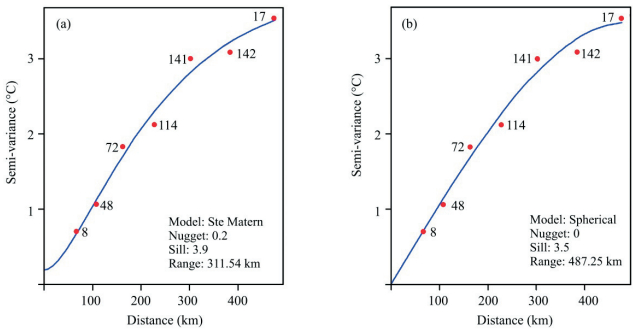
Because they are frequently used for spatial interpolation, both UK with only horizontal coordinates (x and y) as auxiliary predictors, and KED with elevation as an additional auxiliary predictor, were tested and compared for filling the temporal gaps in daily air temperature data. It is critical to choose a proper variogram model and specify its parameters in a Kriging method. In this study, various candidate variogram models were used, including exponential, spherical, Gaussian, and Ste Matern models. The automap package (Hiemstra et al., 2009) in R was used to automatically fit the specified variogram models against the observed samples, and the best one was chosen for interpolation for every day. Results showed that about 63% and 22% of observed daily samples fit the Ste Matern and spherical models best, respectively. The fitted semi-variograms for both models against an observed sample in a selected day are presented in Figure 2.
|
| Figure 2 Fitted semi-variograms for the Ste Matern model (a) and spherical model (b) against an observed sample in a selected day |
In order to assess the efficacy of Kriging spatial interpolation for filling the temporal gaps in daily air temperature data, the estimated values are compared with non-missing observations. At each station we computed two estimates using UK and KED, respectively, for the entire period of record as if all the observations were missing. Then, correlation coefficients between the observed and estimated daily air temperatures were calculated. Performance in terms of root mean square error (RMSE) was also provided. Comparison and assessment for the two selected methods were made on the basis of correlation coefficient and RMSE. The method with higher correlation coefficients and lower RMSEs was used for further analysis.
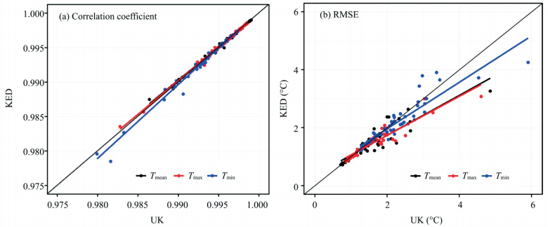
3 Results 3.1 Comparison between the observed and estimated series of daily air temperature dataAt each station, daily series of Tmean, Tmax, and Tmin were estimated by using UK and KED, respectively, as if all the observations at the station were missing. Correlation coefficients and RMSEs between the observed and estimated series were calculated for all the stations, and they are compared in Figure 3. Correlation coefficients between the observed and estimated series during the entire assessing period were > 0.98 at most stations (Table 2). However, there was no notable difference in the correlation coefficients between the two methods. Some RMSEs for the estimated daily air temperature are listed in Table 2. Most RMSEs for the estimated Tmean, Tmax, and Tmin were < 3 ℃, and the RMSEs by KED were significantly smaller than those by UK.
|
| Figure 3 Scatter plots of correlation coefficients and RMSEs between methods UK and KED |
| Items | Method | Correlation coefficient | RMSE (℃) | |||||
| Median | Max | Min | Median | Max | Min | |||
| Tmean | UK | 0.997 | 0.999 | 0.986 | 1.46 | 4.85 | 0.71 | |
| KED | 0.997 | 0.999 | 0.987 | 1.37 | 3.26 | 0.72 | ||
| Tmax | UK | 0.996 | 0.998 | 0.982 | 1.53 | 4.61 | 0.85 | |
| KED | 0.996 | 0.999 | 0.984 | 1.44 | 3.08 | 0.83 | ||
| Tmin | UK | 0.993 | 0.997 | 0.979 | 2.12 | 5.90 | 1.25 | |
| KED | 0.993 | 0.997 | 0.979 | 1.97 | 4.26 | 1.22 | ||
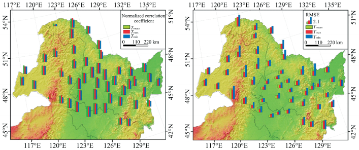
To enlarge the visual difference, correlation coefficients at all stations were normalized and are displayed in the left panel of Figure 4. It is obvious that there was no notable difference in correlation coefficients between the two methods at most stations. The coefficients were smaller at stations near the border or far away from other stations, and in general the coefficients were larger in plain areas than in mountainous areas. The spatial distribution of RMSEs was similar. RMSEs at stations near the border or far away from other stations were very large, while those at stations in plain areas were significantly smaller than those in mountainous areas. In addition, the differences in RMSEs between Tmean, Tmax, and Tmin were notable. RMSEs of Tmin were significantly larger than those of Tmax and Tmean at most stations.
|
| Figure 4 Spatial variation of correlation coefficients and RMSEs between the observed and estimated daily air temperature series from 1960 to 2012 by KED |
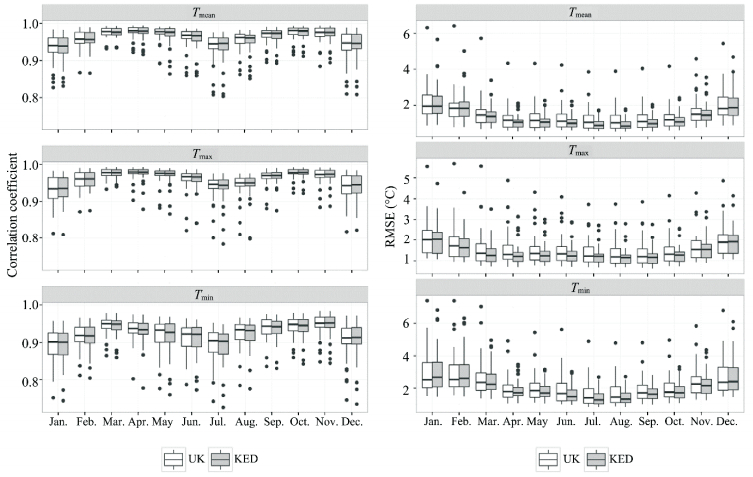
To investigate the temporal variation of the efficacy of Kriging estimation in a year, observed and estimated daily air temperatures in each month in a year from 1960 to 2012 were extracted at each station. The monthly correlation coefficients and RMSEs between the observations and estimations were calculated, and some selected statistics are listed in Tables 3 and 4. Their distribution among all the stations is illustrated as a boxplot in Figure 5. Obviously, there was significant monthly variation in the correlation coefficients and RMSEs.
| Items | Statistics | Method | Jan. | Feb. | Mar. | Apr. | May | Jun. | Jul. | Aug. | Sep. | Oct. | Nov. | Dec. |
| Tmean | Median | KED | 0.939 | 0.956 | 0.976 | 0.979 | 0.976 | 0.967 | 0.946 | 0.961 | 0.973 | 0.979 | 0.975 | 0.946 |
| UK | 0.940 | 0.957 | 0.978 | 0.980 | 0.977 | 0.968 | 0.945 | 0.962 | 0.973 | 0.980 | 0.976 | 0.947 | ||
| 25th percentile | KED | 0.920 | 0.947 | 0.969 | 0.972 | 0.965 | 0.952 | 0.926 | 0.944 | 0.957 | 0.967 | 0.966 | 0.929 | |
| UK | 0.921 | 0.945 | 0.968 | 0.975 | 0.969 | 0.957 | 0.931 | 0.944 | 0.961 | 0.969 | 0.964 | 0.926 | ||
| 75th percentile | KED | 0.960 | 0.975 | 0.986 | 0.988 | 0.985 | 0.977 | 0.960 | 0.968 | 0.979 | 0.987 | 0.987 | 0.969 | |
| UK | 0.960 | 0.976 | 0.986 | 0.988 | 0.985 | 0.978 | 0.961 | 0.970 | 0.980 | 0.987 | 0.987 | 0.970 | ||
| Tmax | Median | KED | 0.936 | 0.961 | 0.978 | 0.980 | 0.976 | 0.966 | 0.944 | 0.951 | 0.970 | 0.979 | 0.974 | 0.946 |
| UK | 0.935 | 0.961 | 0.979 | 0.980 | 0.977 | 0.967 | 0.947 | 0.951 | 0.970 | 0.979 | 0.973 | 0.943 | ||
| 25th percentile | KED | 0.911 | 0.940 | 0.970 | 0.974 | 0.968 | 0.954 | 0.933 | 0.942 | 0.962 | 0.973 | 0.965 | 0.923 | |
| UK | 0.906 | 0.940 | 0.969 | 0.975 | 0.970 | 0.956 | 0.935 | 0.941 | 0.962 | 0.975 | 0.964 | 0.920 | ||
| 75th percentile | KED | 0.964 | 0.979 | 0.986 | 0.986 | 0.983 | 0.975 | 0.958 | 0.963 | 0.979 | 0.986 | 0.984 | 0.969 | |
| UK | 0.965 | 0.978 | 0.986 | 0.986 | 0.983 | 0.975 | 0.958 | 0.962 | 0.977 | 0.986 | 0.984 | 0.970 | ||
| Tmin | Median | KED | 0.901 | 0.918 | 0.949 | 0.934 | 0.927 | 0.922 | 0.903 | 0.932 | 0.943 | 0.946 | 0.952 | 0.914 |
| UK | 0.902 | 0.919 | 0.950 | 0.938 | 0.933 | 0.923 | 0.905 | 0.934 | 0.944 | 0.949 | 0.952 | 0.913 | ||
| 25th percentile | KED | 0.867 | 0.897 | 0.933 | 0.922 | 0.897 | 0.883 | 0.868 | 0.903 | 0.923 | 0.929 | 0.940 | 0.895 | |
| UK | 0.867 | 0.901 | 0.938 | 0.925 | 0.897 | 0.887 | 0.871 | 0.907 | 0.921 | 0.929 | 0.941 | 0.894 | ||
| 75th percentile | KED | 0.921 | 0.940 | 0.958 | 0.951 | 0.949 | 0.940 | 0.922 | 0.946 | 0.957 | 0.962 | 0.968 | 0.940 | |
| UK | 0.923 | 0.940 | 0.960 | 0.952 | 0.949 | 0.939 | 0.926 | 0.948 | 0.961 | 0.962 | 0.968 | 0.938 |
| Items | Statistics | Method | Jan. | Feb. | Mar. | Apr. | May | Jun. | Jul. | Aug. | Sep. | Oct. | Nov. | Dec. |
| Tmean | Median | KED | 1.96 | 1.84 | 1.39 | 1.06 | 1.07 | 1.00 | 0.89 | 0.85 | 0.98 | 1.08 | 1.46 | 1.88 |
| UK | 1.96 | 1.85 | 1.47 | 1.17 | 1.16 | 1.12 | 1.06 | 1.03 | 1.09 | 1.20 | 1.51 | 1.83 | ||
| 25th percentile | KED | 1.44 | 1.33 | 1.01 | 0.77 | 0.77 | 0.79 | 0.70 | 0.71 | 0.78 | 0.84 | 1.10 | 1.33 | |
| UK | 1.43 | 1.32 | 1.01 | 0.79 | 0.77 | 0.79 | 0.73 | 0.72 | 0.77 | 0.85 | 1.09 | 1.34 | ||
| 75th percentile | KED | 2.47 | 2.18 | 1.63 | 1.17 | 1.24 | 1.20 | 1.08 | 1.07 | 1.21 | 1.33 | 1.71 | 2.38 | |
| UK | 2.54 | 2.11 | 1.76 | 1.44 | 1.53 | 1.49 | 1.44 | 1.43 | 1.47 | 1.48 | 1.84 | 2.44 | ||
| Tmax | Median | KED | 2.03 | 1.62 | 1.26 | 1.21 | 1.24 | 1.23 | 1.21 | 1.15 | 1.16 | 1.28 | 1.53 | 1.91 |
| UK | 2.01 | 1.72 | 1.36 | 1.30 | 1.35 | 1.34 | 1.22 | 1.18 | 1.19 | 1.32 | 1.53 | 1.89 | ||
| 25th percentile | KED | 1.34 | 1.17 | 0.95 | 0.96 | 0.96 | 0.98 | 0.94 | 0.89 | 0.88 | 0.96 | 1.13 | 1.35 | |
| UK | 1.35 | 1.17 | 0.99 | 1.03 | 1.01 | 1.00 | 0.93 | 0.89 | 0.89 | 0.98 | 1.13 | 1.35 | ||
| 75th percentile | KED | 2.37 | 2.05 | 1.57 | 1.39 | 1.45 | 1.45 | 1.32 | 1.28 | 1.33 | 1.42 | 1.78 | 2.25 | |
| UK | 2.46 | 2.15 | 1.80 | 1.73 | 1.67 | 1.66 | 1.65 | 1.55 | 1.55 | 1.65 | 1.94 | 2.26 | ||
| Tmin | Median | KED | 2.68 | 2.60 | 2.25 | 1.72 | 1.70 | 1.48 | 1.27 | 1.32 | 1.63 | 1.72 | 2.16 | 2.40 |
| UK | 2.51 | 2.53 | 2.36 | 1.79 | 1.85 | 1.67 | 1.40 | 1.45 | 1.71 | 1.76 | 2.26 | 2.37 | ||
| 25th percentile | KED | 2.02 | 2.07 | 1.81 | 1.50 | 1.47 | 1.22 | 1.02 | 1.08 | 1.30 | 1.37 | 1.66 | 1.85 | |
| UK | 1.98 | 2.05 | 1.79 | 1.42 | 1.42 | 1.21 | 1.04 | 1.09 | 1.34 | 1.43 | 1.67 | 1.86 | ||
| 75th percentile | KED | 3.53 | 3.45 | 2.84 | 2.03 | 2.10 | 1.88 | 1.65 | 1.69 | 1.93 | 2.08 | 2.50 | 3.24 | |
| UK | 3.54 | 3.44 | 2.95 | 2.19 | 2.31 | 2.31 | 1.96 | 2.06 | 2.17 | 2.31 | 2.71 | 3.27 |
|
| Figure 5 Boxplots of monthly correlation coefficients and RMSEs between the observed and estimated daily air temperatures by UK and KED |
The difference in correlation coefficients of the two methods between the observation and estimation was very small. As shown in Table 3 and Figure 5a, the median, 25th percentile, and 75th percentile of the correlation coefficients of Tmean, Tmax, and Tmin were very close to each other by the two methods. The coefficient was highest for Tmean and lowest for Tmin. The boxes for Tmin are significantly longer than those for Tmean, and Tmax, which means the variance in coefficients of Tmin among the 50 stations was highest. The arrangement of boxes for monthly correlation coefficients took an "M" shape (Figure 5a), with lowest values in winter (January and December), highest values in spring and autumn (March, April, October, and November), and moderate values in summer (July). The boxes are also longer in winter and summer than those in spring and autumn.
In contrast to correlation coefficients, the RMSEs between the observations and estimations by the two methods were significantly different. It was obvious that KED was much better than UK for estimating the air temperatures at a given station, because the RMSEs by KED were notably smaller than those by UK at most stations in most times of a year. The magnitude of RMSE varied with the variables. The sequence was Tmean < Tmax < Tmin in the order from the smallest to the largest RMSE. The arrangement of boxes for monthly RMSE takes a "U" shape in Figure 5b, with the largest values in winter (January and December) and the lowest values in summer. The boxes are also longer in winter than those in summer.
4 DiscussionThe correlation coefficients between the observed and estimated daily air temperatures by the two methods did not differ much, while the RMSEs for the estimated Tmean, Tmax, and Tmin by KED were much smaller than those by UK. The medians of RMSE for Tmean, Tmax, and Tmin estimated by KED among the 50 stations were 1.37, 1.44, and 1.97 ℃ during the entire period from 1960 to 2012. The medians of RMSE in most months in a year were < 2 ℃, and were even < 1 ℃ in summer for Tmean. Therefore, Kriging methods were generally desirable for filling temporal gaps of missing data at a given station and spatial interpolation in daily air temperature. However, KED was overall better than UK according to the experiments in this study.
The estimation efficacy of both UK and KED varied in space and time. The spatial variation in estimating performance was mainly controlled by station density and terrain. If there were many meteorological stations in an area and their distances to a given location were small, the estimation uncertainty of air temperature at that location was small. In contrast, if there were few stations around and their distances to the given location were large, the estimation uncertainty at that location was large. For example, in our study the RMSEs at interior stations with more nearby stations were smaller than those at border stations with few, far-away surrounding stations.
The estimation efficacy was also influenced by terrain conditions. In our study the surface conditions of vegetation and terrain (e.g., slope, aspect) were similar among stations in plain areas, which led to similar heating conditions for the air. In the plain areas, without terrain blocking, air masses could move freely and facilitate air heat exchange, which could make the air temperature more homogeneous. Therefore, air temperatures among the different stations changed in a more consistent way than in the mountainous areas. The spatial correlations of air temperature were stronger and the spatial covariances were smaller in the plain areas than the mountainous areas, which resulted in smaller estimated RMSEs in the process of Kriging spatial interpolation.
However, differences in land cover types will influence the local air temperature in plain areas, but this was ignored in this study. Also, in mountainous areas there is strong heterogeneity in surface conditions, which significantly influences heating air. In fractured patches with different aspects and slopes in mountainous areas, the incident solar radiation and ground surface temperatures vary extremely, which leads to critical differences in the local air temperature. Differences in vegetation type and density also have significant influences on the air temperature. In addition, in mountainous regions terrain blocking impedes air mass movement and its heat exchange, which may lead to weaker spatial correlations and larger spatial covariances in air temperature, which in turn lead to higher uncertainties in the spatial interpolation. Thus, to consider the influences of aspect, slope, and land cover type on estimating the local air temperature, Kriging within strata should be used. However, the sparsity of meteorological stations can prevent obtaining reliable semi-variograms within each stratum (Goovaerts, 1997). Therefore, in this study these aspects were not considered.
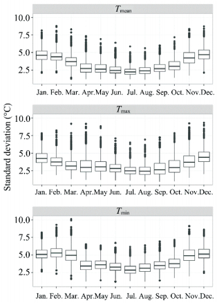
In addition to spatial variation, there was also significant temporal variation in the uncertainty in our Kriging estimations. For example, in our study the estimated RMSEs were smaller in summer and larger in winter, which was mainly caused by the temporal variation in the variance of daily air temperatures among the stations. As shown in Figure 6, the arrangement of boxes for daily air temperature among the 50 stations takes a "U" shape, the same as that for RMSEs in Figure 6. The air temperature variance among the selected stations was bigger in winter than in summer.
|
| Figure 6 Monthly variations in observed daily air temperature |
In this study, we assumed that all the observed air temperatures at a given station were missing and we estimated them from observed samples at surrounding nearby stations by using Kriging methods. However, the assumed missing data at a given station can be used for estimating air temperatures at non-station locations. Generally, the average distance from a non-station location to the nearby surrounding stations was smaller than that from a given station to the nearby surrounding stations. In addition, one more observation is available. Therefore, the estimation uncertainties in air temperatures at non-station locations may be smaller than those presented in this study. However, estimation uncertainties still existed and they were relatively large in winter. The spatial and temporal variation in the estimation uncertainties and their influences on the assessment of permafrost change in the region will be further analyzed in the future.
5 ConclusionThis paper compares the efficacy of KED and UK for filling temporal gaps of missing daily air temperature series from 1960 to 2012 in northeast China by using a cross-validation experiment. Estimations in the entire period of record were made by using UK and KED, respectively, at a given station as if all the observations were missing. Then estimations were compared with the observed air temperatures at each station. Results showed that Kriging methods are desirable for estimating missing values and filling temporal gaps in daily air temperature data. Generally, KED seemed to perform slightly better than UK in this study.
However, the reliability of Kriging methods for estimating air temperature is dependent on a number of factors. The estimation quality is strongly affected by seasonality. In general, estimation uncertainties in air temperature were smaller in summer and larger in winter in the study region, which was mainly caused by the temporal variation of daily air temperature variance among the stations. The estimation quality also had a spatial component. The station density and the distances between them significantly influenced the efficacy. Estimation uncertainties at stations in plain areas densely surrounded by nearby stations were smaller than those in mountainous areas, in large part due to the topographical diversity of the surrounding stations, which led to degradation of spatial coherence among those stations. In areas with complex terrain (borders, mountains), users should be aware of the topographical limitations of the daily estimates.
Acknowledgments:The authors are grateful to the anonymous reviewers for their comments and suggestions on the manuscript. This research was funded by the Chinese National Fund Projects (Nos. 41401028, 41201066) and by the State Key Laboratory of Frozen Soils Engineering (Project No. SKLFSE201201).
| Addink EA, 1999. A comparison of conventional and geostatistical methods to replace clouded pixels in noaa-avhrr images. International Journal of Remote Sensing, 20(5): 961–977. doi: 10.1080/014311699213028 |
| Beck I, Ludwig R, Bernier M, et al, 2015. Assessing permafrost degradation and land cover changes (1986-2009) using remote sensing data over Umiujaq, sub-arctic Québec. Permafrost and Periglacial Processes, 26(2): 129–141. doi: 10.1002/ppp.1839 |
| Bockheim JG, 2015. Global distribution of cryosols with mountain permafrost:An overview. Permafrost and Periglacial Processes, 26(1): 1–12. doi: 10.1002/ppp.1830 |
| Chang XL, Jin HJ, He RX, et al, 2013. Review of permafrost monitoring in the northern Da Hinggan Mountains, Northeast China. Journal of Glaciology and Geocryology, 35(1): 93–100. |
| Christensen N, Wood A, Voisin N, et al, 2004. The effects of climate change on the hydrology and water resources of the Colorado River Basin. Climatic Change, 62(1-3): 337–363. doi: 10.1023/B:CLIM.0000013684.13621.1f |
| Cressie N, 1990. The origins of kriging. Mathematical Geology, 22(3): 239–252. doi: 10.1007/bf00889887 |
| Deutsch CV, Journel AG, 1998. GSLIB:Geostatistical Software and User's Guide, 2nd Edition. New York: Oxford University Press. |
| Diggle PJ, Ribeiro PJ, 2007. Model-based Geostatistics. New York: Springer. |
| Eischeid JK, Pasteris PA, Diaz HF, et al, 2000. Creating a serially complete, national daily time series of temperature and precipitation for the western United States. Journal of Applied Meteorology, 39(9): 1580–1591. doi: 10.1175/1520-0450(2000)039<1580:CASCND>2.0.CO;2 |
| Goovaerts P, 1997. Geostatistics for Natural Resources Evaluation (Applied Geostatistics). New York: Oxford University Press. |
| Guttman NB, 1991. January singularities in the northeast from a statistical viewpoint. Journal of Applied Meteorology, 30(3): 358–367. doi: 10.1175/1520-0450(1991)030<0358:JSITNF>2.0.CO;2 |
| Hengl T, 2007. A Practical Guide to Geostatistical Mapping of Environmental Variables. Italy: European Communities. |
| Hiemstra PH, Pebesma EJ, Twenhofel CJW, et al, 2009. Real-time automatic interpolation of ambient gamma dose rates from the Dutch Radioactivity Monitoring Network. Computers & Geosciences, 35(8): 1711–1721. doi: 10.1016/j.cageo.2008.10.011 |
| Jin H, Hao J, Chang X, et al, 2010. Zonation and assessment of frozen-ground conditions for engineering geology along the China-Russia crude oil pipeline route from Mo'he to Daqing, northeastern China. Cold Regions Science and Technology, 64(3): 213–225. doi: 10.1016/j.coldregions.2009.12.003 |
| Jin H, Luo D, Wang S, et al, 2011. Spatiotemporal variability of permafrost degradation on the Qinghai-Tibet Plateau. Sciences in Cold and Arid Regions, 3(4): 281–305. |
| Jin H, Yu Q, Lü L, et al, 2007. Degradation of permafrost in the Xing'anling mountains, northeastern China. Permafrost and Periglacial Processes, 18(3): 245–258. doi: 10.1002/ppp.589 |
| Kandasamy S, Baret F, Verger A, et al, 2012. A comparison of methods for smoothing and gap filling time series of remote sensing observations:Application to modis lai products. Biogeosciences Discuss, 9(12): 17053–17097. doi: 10.5194/bgd-9-17053-2012 |
| Luo D, Jin HJ, Marchenko S, et al, 2014a. Distribution and changes of active layer thickness (alt) and soil temperature (ttop) in the source area of the Yellow River using the Gipl model. Science China Earth Sciences, 57(8): 1834–1845. doi: 10.1007/s11430-014-4852-1 |
| Luo D, Jin H, Jin R, et al, 2014b. Spatiotemporal variations of climate warming in northern northeast China as indicated by freezing and thawing indices. Quaternary International, 349: 187–195. doi: 10.1016/j.quaint.2014.06.064 |
| Meng Q, Liu Z, Borders BE, 2013. Assessment of regression kriging for spatial interpolation-comparisons of seven GIS interpolation methods. Cartography and Geographic Information Science, 40(1): 28–39. doi: 10.1080/15230406.2013.762138 |
| Rossi RE, Dungan JL, Beck LR, 1994. Kriging in the shadows:Geostatistical interpolation for remote sensing. Remote Sensing of Environment, 49(1): 32–40. doi: 10.1016/0034-4257(94)90057-4 |
| Sannel ABK, Hugelius G, Jansson P, et al, 2016. Permafrost warming in a subarctic peatland-which meteorological controls are most important?. Permafrost and Periglacial Processes, 27(2): 177–188. doi: 10.1002/ppp.1862 |
| Serreze MC, Walsh JE, Chapin FS, et al, 2000. Observational evidence of recent change in the northern high-latitude environment. Climatic Change, 46(1): 159–207. doi: 10.1023/a:1005504031923 |
| Stooksbury DE, Idso CD, Hubbard KG, 1999. The effects of data gaps on the calculated monthly mean maximum and minimum temperatures in the continental United States:A spatial and temporal study. Journal of Climate, 12(5): 1524–1533. doi: 10.1175/1520-0442(1999)012<1524:TEODGO>2.0.CO;2 |
| Wackernagel H, 2003. Multivariate Geostatistics:An Introduction with Applications, 2nd Edition. Springer-Verlag. |
| Wei Z, Jin H, Zhang J, et al, 2011. Prediction of permafrost changes in northeastern China under a changing climate. Science China Earth Sciences, 54(6): 924–935. doi: 10.1007/s11430-010-4109-6 |
| Weiss DJ, Atkinson PM, Bhatt S, et al, 2014. An effective approach for gap-filling continental scale remotely sensed time-series. Isprs Journal of Photogrammetry and Remote Sensing, 98: 106–118. doi: 10.1016/j.isprsjprs.2014.10.001 |
 2016, 8


