Article Information
- Abbas Tanveer, Nabi Ghulam, W. Boota Muhammad, Hussain Fiaz, I. Azam Muhammad, Jun Jin Hui, Faisal Muhammad . 2016.
- Uncertainty analysis of runoff and sedimentation in a forested watershed using sequential uncertainty fitting method
- Sciences in Cold and Arid Regions, 8(4): 297-310
- http://dx.doi.org/10.3724/SP.J.1226.2016.00297
Article History
- Received: April 09, 2016
- Accepted: June 01, 2016
2. State Key Laboratory of Frozen Soils Engineering, Cold and Arid Regions Environmental and Engineering Research Institute, Chinese Academy of Sciences, Lanzhou, Gansu 730000, China
Water is the most precious and primary natural resource and a major constituent of all living matter on the planet Earth. It is a vital factor for economic development and augmenting the growth of agriculture and industry, especially in the perspective of rapidly increasing population and urbanization. Many developing zones face scarcity of fresh water. Thus, the availability and sustainable use of water resources have become the core of local and national strategies and politics in these regions. The behavior of each process in a catchment is controlled by its own characteristics as well as by its interaction with other processes active in the catchment. The predominant hydrologic processes include rainfall, interception, evapotranspiration, infiltration, surface runoff, percolation, and subsurface flow.
Soil erosion caused by anthropogenic intervention is posing a severe challenge to the productivity of land by the loss of fertile soil and to the life of reservoirs by the deposition of sediment. The process of soil erosion and sediment transport and deposition are nonlinearly related to the causal factors and are highly variable both spatially and temporally (White, 2005). Monitoring of these processes is quite complex and expensive. Modeling provides an alternative approach for estimation of sediment yield and also to achieve a better understanding of sediment movement and delivery. In recent years, some of the prominent models, like the Universal Soil Loss Equation (USLE) and its modifications - the Modified USLE (MUSLE) and the Revised USLE (RUSLE)- are increasingly being used. Assessing and mitigating soil erosion at the watershed level is complex both spatially and temporally. Hence, watershed models that are capable of capturing these complex processes in a dynamic manner can be used to provide an enhanced understanding of the relationship between hydrologic processes, erosion/sedimentation, and management options.
In recent times, many mathematical models have incorporated the GIS application to generate inputs and display output or as an interface for the entire modeling process. It has added confidence in the accuracy of modeling by providing a more practical approach toward the watershed conditions, defining watershed characteristics, improving the efficiency of the modeling process, and ultimately increasing the estimation capabilities of hydrological modeling (Bhuyan et al., 2003). The Soil Water Assessment Tool (SWAT) model is a watershed model that analyzes the impact of land management practices on water, sediment, and agricultural chemical yields in large, complex watersheds. It is extensively applied in many parts of the world. A comprehensive review of SWAT model applications is given by Gassman et al.(2007a, b).
Hydrologic models frequently contain many parameters that cannot be measured as they are time-consuming, costly, and sometimes hard to access, so inverse modeling has become a main method for calibration (Beven and Binley, 1992). SUFI-2(sequential uncertainty fitting method) is a semi-automated algorithm that permits users to interface with it iteratively. Also, this strategy has high computational efficiency and has been progressively utilized in recent years (Abbaspour et al., 2007; Rostamian et al., 2008). Abbaspour et al.(1997)described a few features of SUFI-2 in detail. They disclosed that SUFI-2 represents a parameter estimation procedure that is sequential, operates within parameter uncertainty domains, employs only forward calculations, and is iterative in nature. SUFI-2 application areas include streamflow simulation (Setegn et al., 2008), hydrology and water quality simulation (Abbaspour et al., 2007), sediment modeling (Talebizadeh et al., 2010), and freshwater availability (Schuol et al., 2008). Therefore, SUFI-2 was used in this study for model calibration and uncertainty analysis.
Simly is the largest reservoir of drinking water for people living in Islamabad, the capital of Pakistan. Up to 47 million gallons per day (MGD) of water is supplied to the Capital Development Authority from Simly Dam. Reduced inflow of water to the Simly Dam has reduced the withdrawal of water for human use. At present, approximately 64 MGD of water is being produced against the demand of around 81 MGD. The live storage capacity of Simly Dam is continuously declining due to sedimentation in the reservoir, and the inflows to the Simly reservoir in dry years are almost half those of wet years. Thus, the problem will be more complex in dry years in the future.
The use of computer models for modeling the hydrological processes of the Simly watershed can be of great help to watershed management authorities in developing a suitable management programme. The objective of modeling the Simly Dam watershed in the Soan River Basin was to set up and calibrate the adapted model. This made it possible to predict the response at the outlet of the watershed in order to develop an efficient decision framework to facilitate, plan, and assess the management of this crucial reservoir.
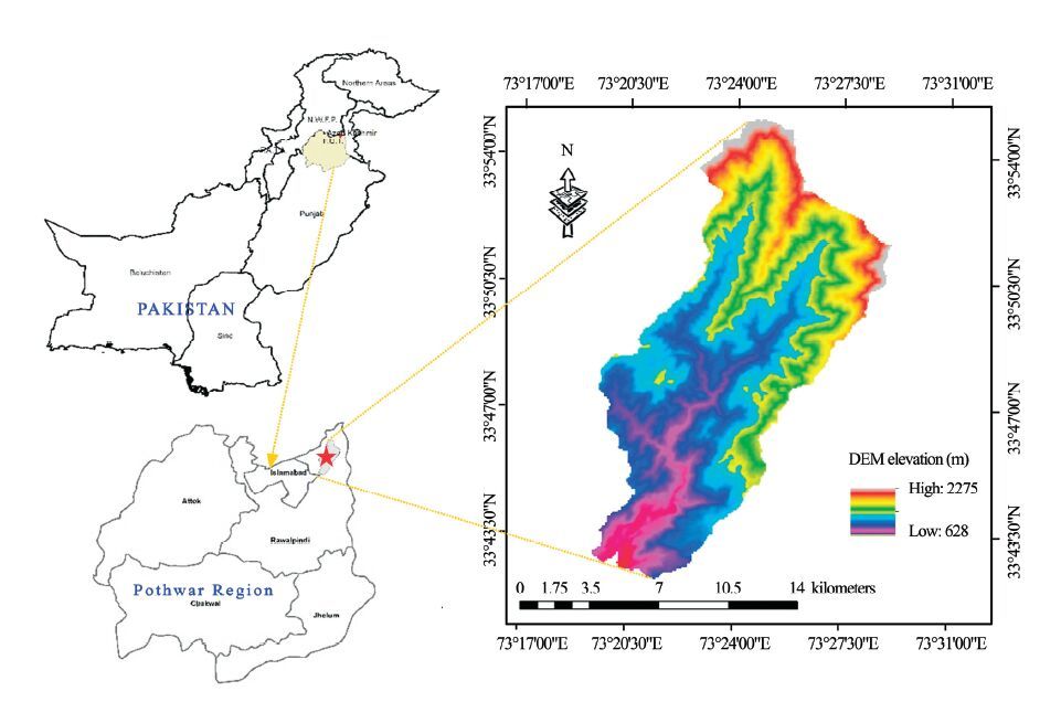
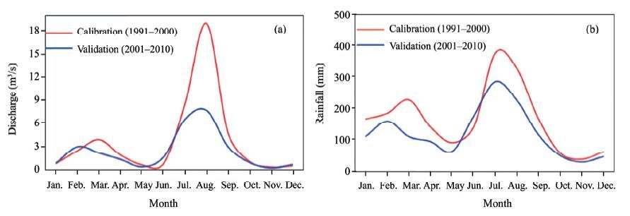
2 Study areaThe study was conducted in a small watershed in the Soan River Basin in the central part of the Pothwar Plateau in northern Pakistan. The watershed, which has a drainage area of 159 km2, is located 19 miles east of Islamabad, the capital of Pakistan (Figure 1). The watershed drains its water to the Simly reservoir, which was constructed to supply water to the capital city. The area is located between 33°43'41.33"N- 33°53'37.5"N and 73°20'22.09"E-73°23'19.50"E. The elevation of the watershed ranges from 690 to 2, 261 m a.s.l. and rises steadily from south to north. The topography of the study area is hilly. The land covers are forests (49.74%), vegetation/agriculture land (16.87%), built-up areas (4.32%), water bodies (3.27%), rangeland (8.84%), and barren land (16.95%). The climate in the study area has two distinct seasons: a wet season (June to September) and a dry season (October to May). The coldest month is January when the mean maximum temperature is 17.7 ℃ and the minimum can reach −5 ℃. From February to May the temperature rises 5 ℃ per month, and the highest temperatures are recorded in June, when they may rise to 40 ℃ in the lower portion of the study area near Islamabad. The watershed receives an annual rainfall of 1, 774 mm. Five main river tributaries contribute to the Simly reservoir, the Soan, Khad, Mangal, Basant, and Bissa rivers. During 28 years of records (1983-2010), the mean monthly flows at the outlet varied between 0.61 m3/s (minimum) to 11.98 m3/s (maximum), and the average annual flows varied between 1.6 m3/s (minimum) to 7.9 m3/s (maximum). The average monthly rainfall and discharge data are shown in Figure 2.
|
| Figure 1 Location of study area |
|
| Figure 2 Average monthly (a) discharge for calibration and validation, and (b) rainfall for calibration and validation |
The SWAT (Soil and Water Assessment Tool) is a physically-based, continuous-time hydrologic model developed by the U.S. Department of Agriculture (USDA), Agricultural Research Service (ARS). The key objective associated with SWAT is to envisage the impact of land management activities or agriculture on water, sediment, and agricultural chemical yields in ungauged basins. The SWAT model allows simulation by simply dividing the watershed into a number of sub-watersheds. The major components consist of climate conditions, erosion, hydrology, plant growth, land management, pesticides, nutrients, and stream routing. Further detailed description of SWAT can be found in the study by Nietsch et al.(2005).
Each sub-basin in SWAT is discretized into a series of hydrological response units (HRUs), which are unique in their soil-land use-slope combinations (Abbaspour et al., 2007). In this work, surface runoff was estimated based on the USDA's Soil Conservation Service curve number procedure (USDA Soil Conservation Service, 1972), which requires only daily precipitation data and does not assume soil profile homogeneity, as considered by the Green-Ampt method (Green and Ampt, 1911). In the routing phase, SWAT uses Manning's equation to calculate the rate and velocity of flow. Owing to limitations in the Muskingum routing method in SWAT (Kim and Lee, 2010), we used the variable storage method (Williams, 1969) for flow routing through the channel.
The hydrological cycle simulated by SWAT is based on following equation:
where SWtis the final water content (mm), SW0 is the initial water content (mm), t is the time (days), Rdis the rainfall on some specific i day (mm), Qsurf is the runoff on day i(mm), Ea is the amount of evapotranspiration on day i(mm), Wsep is the amount of percolation in the soil profile on day i(mm), and Qgw is the amount of return flow on day i(mm).
SWAT provides a couple of methods for surface runoff estimation: the SCS method (USDA Soil Conservation Service, 1972) and the Green & Ampt infiltration technique (Green and Ampt, 1911). Applying daily or sub-daily rainfall, SWAT simulates surface runoff amounts as well as optimum runoff for each HRU. The SCS curve number equation is:
in which Qsurf is the cumulative runoff or rainfall excess (mm), Rday is the rainfall depth for any day (mm), and S is the retention parameter (mm). The retention parameter is defined by:
Sediment yield is estimated for each sub-basin with the modified universal soil loss equation (MUSLE) (Williams, 1975):
where Sed is defined as the sediment yield rate (t/d), Qsurf is the surface runoff volume (mm/d), qpeak is the peak runoff rate (m3/s), Areahru is the area of the HRU (ha), KUSLEis the USLE soil erodibility factor, CUSLE is the USLE crop management factor or cover management factor, PUSLE is the USLE support practice factor, LSUSLE is the USLE topographic factor, and CFRG is the coarse fragment factor.
3.2 Sequential uncertainty fitting (SUFI-2)In SUFI-2, the uncertainties are calculated from all the sources, such as rainfall data, soil data, land use data, observed data, and parameters. The output uncertainty of the model, quantified by a 95% prediction uncertainty (95PPU, known as the p-factor) is calculated at the 2.5% and 97.5% levels of the cumulative distribution of an output variable (Yang et al., 2007). The p-factor ranges from 0 to 1. Another factor used to quantify the uncertainty analysis is the r-factor, which is the average width of the 95PPU band divided by the standard deviation of the observed values. The r-factor ranges from 0 to infinity. A p-factor of 1 and an r-factor of 0 is a simulation that exactly equals the observed data, which is an ideal but impossible case due to uncertainties from the measurements and other different sources. A higher value of the p-factor can be attained at the cost of a higher r-factor. Thus, a balance must be achieved between the two factors, which will result in decreasing parameter uncertainty. When satisfactory values of these factors are attained, the reduced parameter uncertainty ranges are the preferred ones (SWAT-CUP, 2015).
SUFI-2 works by performing a few iterations, typically less than five. In every iteration the parameter extents get smaller, which creates better results in the next iteration. As the parameter extents get smaller, the 95PPU envelope gets smaller, leading to a smaller r-factor and p-factor (SWAT-CUP, 2015. In the case of good-quality observed data, 80%~100% of the observed data is captured by the corresponding 95PPU band, whereas low-quality observed data might be adequate enough to capture 50% of the observed data by the 95PPU. The average thickness of the 95PPU band () and the r-factor are calculated by Equations (5) and (6):
where
Applying SUFI-2 includes the following steps:(1) First, the objective function and meaningful parameter ranges are defined;(2) Latin Hypercube sampling is conducted, the corresponding objective functions are evaluated, and the sensitivity matrix and parameter covariance matrix are calculated;(3) the 95% predictive interval of a parameter is computed; and (4) the 95PPU, p-factor, and r-factor are calculated. The p-factor ranges between 0 and 1, whereas the r-factor ranges between 0 and infinity. The goodness of calibration and the prediction uncertainty are judged on the basis of the closeness of the p-factor to 1 and the r-factor to 1 (Yang et al., 2007).
3.3 Elevation bandsElevation is considered one of the most important variables related to meteorological parameters (Zhang et al., 2008), particularly temperature and snow amount. Sub-watershed temperatures and precipitation are adjusted within each elevation band based on the difference between the elevation of the sub-watershed meteorological station and each elevation band multiplied by the lapse rate (Fontaine et al., 2002; Neitsch et al., 2011). Here, five elevation bands were used to adjust the temperature and rainfall based on sub-basin elevation variation.
3.4 Model data inputFor hydrological modeling, long-term datasets of daily rainfall, minimum and maximum temperature, wind speed, and humidity are required. The Simly watershed has only one weather station in the Murree District, installed by the Pakistan Meteorological Department (PMD). These datasets for the years 1983-2010 were collected from the PMD and were processed according to the model input format. Because hydrological data were required for the calibration and validation of the model for the Soan River, the observed flows data covering the years 1983-2012 were collected from the Capital Development Authority (CDA) in Islamabad. The elevation data in raster format had a resolution of 30m×30m and were provided by the U.S. National Elevation databases. Sub-basin delineation and stream network characteristics were derived from the DEM. The land cover map was prepared by the supervised classification method of Landsat images with spatial resolution of 30 m (downloaded from U. S. Geological Survey (USGS) Landsat datasets). The soil map was obtained from IPCC global soil classes developed by the Food and Agriculture Organization of the United Nations (FAO) database. The necessary input information required by the SWAT model was extracted from the same database for the soil type, namely, soil texture, hydrological soil group (HSG), soil depth, rock fragments, and organic carbon content. The list of data type, sources, and description is given in Table 1.
| Data type | Source | Resolution | Description |
| Topography | U.S. Geological Survey (USGS) | 30 m | Topographic data, DEM (elevation) |
| Land use | Developed from Landsat TM data | 30 m | Classified land use such as forest, agriculture, crops, water, etc. |
| Soil | Food and Agriculture Organization of UN (FAO) | - | Classified soil and physical properties such as sand, silt, clay, bulk density, etc. |
| Climate | Pakistan Metrological Department (PMD) | - | Precipitation, temperature, solar radiation, wind speed |
| Hydrology | Capital Development Authority (CDA), Islamabad | - | River discharge, sediment data |
The model performance was evaluated using three well-known statistical criteria, the coefficient of determination (R2), the Nash-Sutcliffe efficiency (NS), and percent bias (PBIAS). The R2 ranges from 0 to 1 with higher values indicating less error variance; the NS estimates how well the plot of observed versus simulated data fits the 1:1 line; and PBIAS has the ability to measure the average tendency of the simulated data to be larger or smaller than the observed data. Low values of PBIAS indicate accurate model simulation, positive values indicate model underestimation, and negative values indicate model overestimation bias (Gupta et al., 1999). The values of R2, NS, and PBIAS are determined by these equations:
where Oi = observed value;O= mean observed value; Si = simulated value; and S= mean simulated value (Santhi et al., 2001).
3.6 Model setupFirst the watershed was delineated and subdivided into nine sub-basins. A user look-up table was prepared for the land use and soil map to identify the SWAT code. Land use, soil type map, and slope were classified by the Arc SWAT. The sub-basins were further divided into units of unique soil/land use/slope characteristics called hydrological response units (HRUs), based on dominant land use, soil type, and slope using a threshold of 3% for land use, 3% for soil type, and 3% for slope. These HRUs are defined as homogeneous spatial units characterized by similar geomorphologic and hydrological properties (Flugel, 1995). This process resulted in 114 HRUs within the nine sub-basins. The total number of HRUs should be sufficient to account for the various hydrological conditions in the watershed, and at the same time limited enough to reduce the input data requirements and improve the modeling efficiency (Qiu and Wang, 2014).
The dissemination of land use, soil, and slope individualities inside of each HRU have the greatest effect on the stream flow. As the percentage of the threshold value of land use, slope, and soil expands, the actual evapotranspiration starts decreasing because of eliminated land use classes. Thus, HRU characteristics are the key variables influencing the stream flow. Here, surface runoff was computed utilizing the modified Soil Conservation Service curve number method. Channel routing was estimated by the variable storage method.
The observed data were obtained from 1990 to 2010. Latin Hypercube One-at-a-Time (LH-OAT) sensitivity analysis was performed using data from 1991-2000 to identify key parameters required for calibration. The data from 1987 to 2000 were used for calibration, and the remaining 10 years of data were used for validation, with 4 years of data (1987-1990) as a warm-up period.
4 Results and discussion 4.1 Sensitivity analysisThe LH-OAT method (Van Griensven et al., 2006) was used for the catchment area, using 20 hydrological parameters. The upper- and lower-bound parameter values were taken from the SWAT user manual (Neitsch et al., 2005). Out of 24 parameters (Table 2), 19 were considered for the model calibration. The remaining parameters caused no significant changes in the output results and were not considered in the auto-calibration procedure.
| Rank | Parameter Name | Iteration 1:Default parameter ranges | Iteration 2:Modified parameter ranges | Iteration 3:Fitted parameter ranges |
| 1 | CN2.mgt | −0.98, 0.01 | −0.88, −0.29 | −0.75, −0.44 |
| 2 | HRU_SLP.hru | 0.01, 0.25 | 0.14, 0.26 | 0.13, 0.22 |
| 3 | GW_DELAY.gw | 218, 594 | 405, 779 | 140, 460 |
| 4 | SMFMX.bsn | 4.20, 12.80 | 7.60, 14.36 | 0.80, 6.80 |
| 5 | TLAPS.sub | −4.60, −8.20 | −6.39, −7.60 | −6.50, −6.70 |
| 6 | CH_K2.rte | 39.00, 73.00 | 10.10, 90.88 | 26.50, 51.70 |
| 7 | TIMP.bsn | 0.20, 0.70 | −0.02, 0.477 | −0.18, 0.25 |
| 8 | SMTMP.bsn | −2.00, 3.40 | 2.12, 4.87 | 2.50, 4.23 |
| 9 | SFTMP.bsn | −1.60, 5.00 | 1.04, 6.41 | 1.60, 4.81 |
| 10 | SOL_AWC.sol | −0.10, 0.04 | −0.03, 0.08 | 0.02, 0.15 |
| 11 | GWQMN.gw | 0.07, 1.30 | 0.60, 1.78 | 0.90, 2.10 |
| 12 | SOL_BD.sol | −0.50, 0.20 | −0.28, 0.16 | −0.24, 0.024 |
| 13 | SLSUBBSN.hru | 0.06, 0.20 | 0.06, 0.16 | 0.04, 0.12 |
| 14 | OV_N.hru | −0.10, 0.02 | −0.18, −0.04 | −0.12, 0.09 |
| 15 | USLE_C | 0.004~0.320 | 0.001~0.200 | 0.003~0.450 |
| 16 | USLE_P | 0.1~1.0 | 0.2~0.7 | 0.5~0.8 |
| 17 | CH_Eros | 0.00~1.00 | 0.04~0.30 | 0.01~0.10 |
| 18 | SPCON | 0.0001~0.0100 | 0.0001~0.0070 | 0.0001~0.0010 |
| 19 | SPEXP | 1.0~1.5 | 1.0~1.3 | 1.3~1.4 |
Initially, 7 snow parameters were utilized in the LH-OAT procedure: maximum melt factor SMFMX, snowmelt base temperature SMTMP, snowfall temperature threshold SFTMP, minimum melt factor SMFMN, snowpack temperature lag TIMP, areal snow coverage threshold at 100% SNOCOVMX, and areal snow coverage threshold at 50% SNO50COV. Out of these seven parameters, the first five were ranked among the top 10.
Four dominant parameters included CN2, HRU_SLP, GW_DELAY, and SMFMX. CN2 is the rainfall runoff conversion coefficient. An increase or decrease in the CN2 value will directly result in an increase or decrease of surface runoff. The average slope steepness HRU_SLP controls the speed of the water from upstream to downstream. A high slope gradient means rapid flow of water, whereas a low slope gradient indicates a more nearly level stream bed and sluggishly moving water. Most of the catchment area had a very strong slope gradient, between 30% and 50%. Thus, this parameter had a great influence on the model output.
Of the 7 snow-related parameters, the model was most sensitive to the four snowmelt parameters SMFMX, TIMP, SMTMP, and SFTMP. This was reasonable because the area is located at the outer Himalayas and features a tropical highland climate. The area receives heavy snowfall during December-March, with an average value of 120 mm. A substantial portion of runoff water is contributed by the snowmelt in this region.
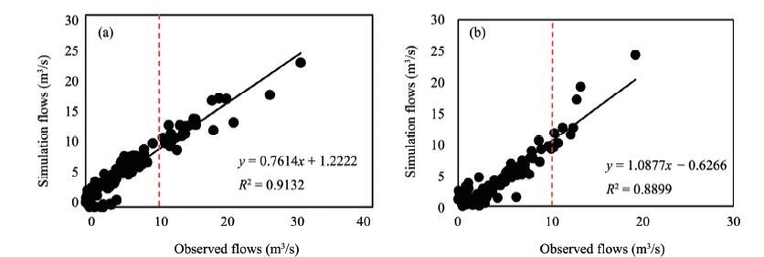
4.2 Model calibration and validationThe parameters analyzed during the sensitivity analysis were also used during the auto-calibration procedure. In the SUFI-2 algorithm, 1, 000 simulations were performed in each iteration. The same simulation numbers were used in the validation. The calibration and validation statistics are given in Table 3, which shows the model calibration results for the 10-year period 1990-2000. Overall, the model performance was efficient in monthly simulation, with an NS value of 0.85 and an R2 value of 0.91 (Figure 3), with a lower value of PBIAS = 2.1%. The results showed that there was good agreement between the observed and simulated flows. The calibrated model was then run from 2001-2010 to validate the model. The validation statistics also displayed satisfactory model performance, with an NS value of 0.84 and an R2 value of 0.89 (Figure 3), with PBIAS = 5.88%.
|
| Figure 3 Scatter plots of best-simulated and observed runoff with 95PPU during calibration (a) and validation (b) period (2001-2010) |
| Performance indices | Calibration (1991-2000) | Validation (2001-2010) |
| R2 | 0.91 | 0.88 |
| NS | 0.85 | 0.84 |
| PBIAS(%) | 2.10 | 5.88 |
| p- factor | 0.72 | 0.67 |
| r- factor | 0.81 | 0.68 |
A plot of the monthly simulations for the validation period showed that the observed and simulated runoff closely matched, except for some overestimation during some high-flow events. Analysis of monthly simulated and observed flows for the calibration and validation showed that the SWAT was unable to model the high flows. This poor performance during high-flow events has been reported by many researchers (e.g., Nyeko, 2010; Jajarmizadeh et al., 2012; Qiu et al., 2012). This might happen because when several storms occur in a single day, the curve number and soil moisture change from storm to storm (Kim and Lee, 2008). However, the SCS-CN technique characterizes a rainfall event as the sum of all rainfall that occurs during single day, and this may lead to insufficiency in modeling high flows (Choi et al., 2002). Likewise, SWAT overestimates the monthly streamflow during the summer and spring seasons due to greater rainfall variability, and underestimates streamflow during extreme rainfall events (Srinivasan, 1998).
In our study the SWAT model underestimated flows throughout the calibration and validation periods. This may have been due to a deficiency in modeling snowmelt runoff processes (Fontaine et al., 2002), or the lack of a good network of climate stations. Other possible reasons could be the general issues of hydrological modeling, such as an incomplete soil and land use database or inaccurate GIS information (Wu and Chen, 2014). Nevertheless, the overall result demonstrated that SWAT was able to simulate the hydrological characteristics of the Simly watershed very well.
Monthly sediment yield at the outlet of the watershed was simulated for the whole watershed. Model performance for simulating the sediment yield was evaluated using a given set of criteria. The important parameters influencing sediment were changed to improve agreement between the observed and simulated sediment. During calibration of the model, the final set of parameters signified the characteristics of the watershed. The calibration procedure considerably reduced the variation between the measured and simulated sediment load. The sediment yield from a watershed is associated with the complicated interaction between land use, soil, vegetation, and topography (Singh et al., 2014). The sediment parameters contemplated during the calibration based on the LH-OAT sensitivity analysis were the USLE C variable for water erosion related to land use, the USLE support practice variable, a parameter for computing the maximum possible amount of sediment that will be produced throughout channel sediment routing, the channel erodibility variable, and an exponent parameter for computing sediment produced in channel sediment routing. These parameters were adjusted to particular levels in different iterations where they were able to signify the features of the present land use and topography of the watershed.
Rainfall and runoff are the main contributing factors for the detachment, transport, and deposition of sediment particles. During the onset of the monsoon (in the study area, the first week of June), most of the water is lost through infiltration and other losses, thereby reducing sediment yield at the outlet. In fact, sediment concentration increased rapidly during June, and sediment yield and runoff reached their peaks in September. Higher values of sediment yield were observed during August and September for both the calibration and validation periods.
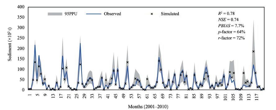
Overall, the performance of the model for sediment modeling was efficient. The R2 and NS values obtained were 0.81 and 0.79, respectively, during the calibration period. The calibrated model was validated for the years 2001-2010. The model performance criteria given in Table 4 for the validation period (2001-2010) indicate the coefficient of determination, R2 = 0.78 and NS = 0.74, which demonstrate that the model closely predicted the observed values of sediment yield.
4.3 Uncertainty analysis of runoff modelingSUFI-2 analysis begins with wide but meaningful ranges of parameters, and most of the observed flows fall under the 95PPU band with higher uncertainties. However after a few iterations, this uncertainty is reduced. To adjust parameters, three different methods are used:(1) replacing the existing value of a parameter;(2) multiplying (1 + a given value) with the existing value; or (3) adding value to the existing parameter value. The parameters used in the first iterations were based on information available in the study area.
In SUFI-2 each iteration provides the best parameters and suggests new ranges. In each iteration new estimated parameters are exported and used for the next iteration. When calibrating a model, one should always be cautious about the final range of the adjusted parameters, as they should always be meaningful and should represent the subject's characteristics (Talebizadeh et al., 2010). Some parameters are not well estimated and have no physical meaning, and therefore need to be manually adjusted to make them not go beyond the maximum/minimum range values. In our study the suggested ranges of some of the other parameters were further adjusted to agree with the physical meaning and the requirements of the SWAT model. For example, the value of the groundwater delay time was adjusted to 150 days in the third iteration. This parameter represents the time lag when that water exits the soil profile and enters the shallow aquifer. The curve number was adjusted within the range ±40% from the curve number value for moisture condition Ⅱ.
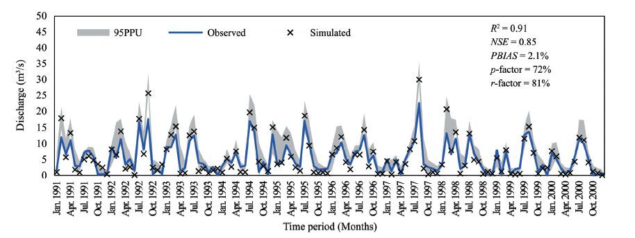
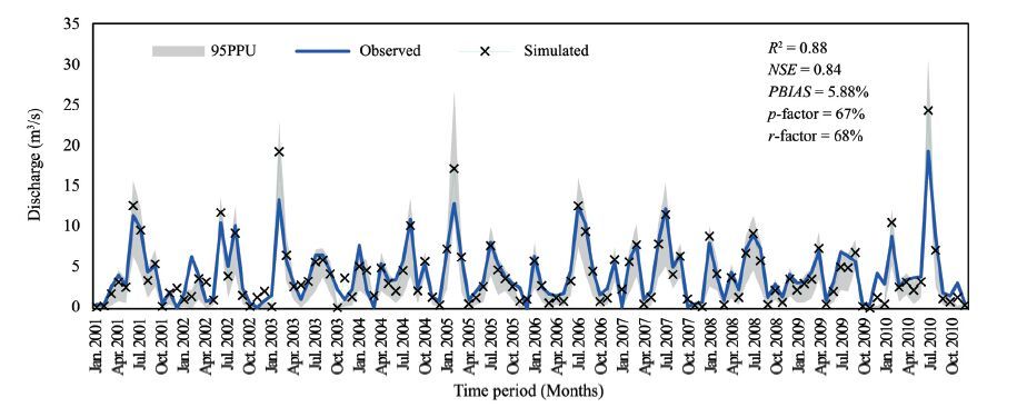
The uncertainty analyses with SUFI-2 for both the calibration and validation periods are shown in Figures 4 and 5. The green region is the 95% prediction interval for the parameter set of the best estimation, and it covers most of the flows during the calibration and validation periods.
|
| Figure 4 The best-simulated and observed runoff with 95PPU during calibration period (1991-2000) |
|
| Figure 5 The best-simulated and observed runoff with 95PPU during validation period (2001-2010) |
The p-factor for the calibration was observed to be 0.72, meaning that 72% of the observed data was captured by the corresponding 95PPU; the r-factor was 0.81. In the validation period, 67% of the observed flows were captured by 95PPU and the r-factor was 0.68. The reduction in p-factor from 72% to 67% during validation was a clear indication of the uncertainties from the different input variables, such as rainfall. Previous studies have reported p-factors ranging from 4.2% (Li et al., 2009) to 96.5% (Zhang et al., 2009) and r-factors from 0.26 to 0.94 (Gong et al., 2010; Narsimlu et al., 2015) at the monthly time scale. The p-factors in this study during calibration (80%) and validation (65%) were within the reported ranges of p-factors, while the r-factors ranging from 0.68 to 0.85 in this study were slightly higher than the reported ranges.
Careful examination of the calibration results (Figure 4) illustrates that peak flows were not captured by the corresponding 95PPU band, which was the primary source of uncertainty during the calibration process. Then during the validation interval this behavior changed and most of the low flows were not captured by the 95PPU band, although all of the high flows were nicely captured during the validation period. Very low or zero base flows during dry periods could have led to smaller p-factors during the validation period. Scatter plots for calibration and validation revealed that the SWAT model had been calibrated with observed flows varying from 0~30 m3/s, whereas during validation most of the observed flows were less than 10 m3/s. The low-flow conditions during the validation might be why most of the low flows were not captured by the 95PPU band. It is important to mention here that several previous studies have reported that SWAT model has deficiencies in simulating groundwater flows (e.g., Rostamian et al., 2008).
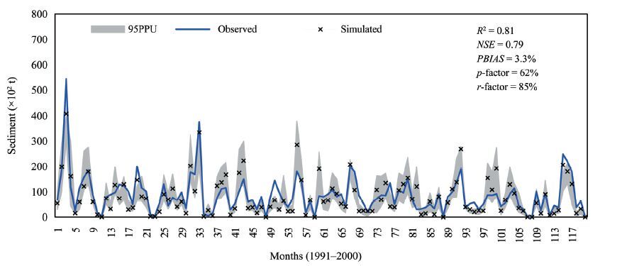
4.4 Uncertainty analysis of sediment modelingThe calibration results of monthly sediment analysis for the Simly watershed are shown in Figure 6. The p-factor for the calibration was 0.62, meaning 62% of the observed sediment data was captured by the corresponding 95% prediction interval. The r-factor was 0.85. Similar to the runoff calibration, the peak sediment values were not mostly captured by the 95PPU band. The reasons could be poor accuracy of the measured data and the dispersed nature of the data. Tolson and Shoemaker (2004)calibrated and validated a SWAT model for prediction of dissolved and particulate phosphorus transport, and also flow and sediment transport, against a large set of monitoring data. As in our case, they reported that the largest error in model predictions for sediment loading was always associated with peak flow prediction errors. As Abbaspour et al.(2007)discuss, the "second storm effect" may also be partly responsible for poor sediment results. After a storm, there is less sediment to be moved, and the remaining surface layer is much more difficult to mobilize. Hence, a similar size storm, or even a bigger size second or third storm could actually result in smaller sediment loads. The model, however, does not account for this effect as overestimates the load Abbaspour et al.(2007).
|
| Figure 6 The best-simulated and observed sediment yield with 95PPU during calibration period (1991-2000) |
Despite these shortcomings, we found the results quite useful. The validation results for sediment are shown in Figure 7, where large uncertainties can be seen. For validation, 65% of the observed sediment data was captured by the 95PPU band (Table 4). The r-factor was 72%. The results indicated a better estimation of sediment yield in the validation process, bracketing 3% more observed sediment data as compared to the calibration process. The model mostly shows large uncertainties at extreme events during the calibration and validation periods.
|
| Figure 7 The best-simulated and observed sediment yield with 95PPU during validation period (2001-2010) |
| Performance indices | Calibration (1991-2000) | Validation (2001-2010) |
| R2 | 0.81 | 0.78 |
| NS | 0.79 | 0.74 |
| PBIAS(%) | 3.40 | 7.70 |
| p-factor | 0.62 | 0.64 |
| r-factor | 0.85 | 0.72 |
The results indicated that the model performance indices for sediment yield were somewhat less than those for runoff. Several other researchers have also reported that the SWAT model performs better for runoff than sediment yields (e.g., Kaur et al., 2003; Tripathi et al., 2005; Behera and Panda, 2006).
The results of this study can be further assessed, keeping in view the unreliability of the input data. The parameter values derived from various sources need to be verified in the field, but this is a difficult task in view of the study area's difficult access and being mostly covered by thick forest. Similarly, the land use derived from remote sensing data was based on unsupervised classification. Further, the rainfall, runoff, and sediment yield data used in this study may have involved a number of possible human and instrumental errors. In view of all this, it can be concluded from the simulation results of our study that the SWAT model simulated the runoff and sediment yield reasonably well from an intermediate watershed in the Himalayan region. The performance of the model could possibly be enhanced with some refinement in the input data.
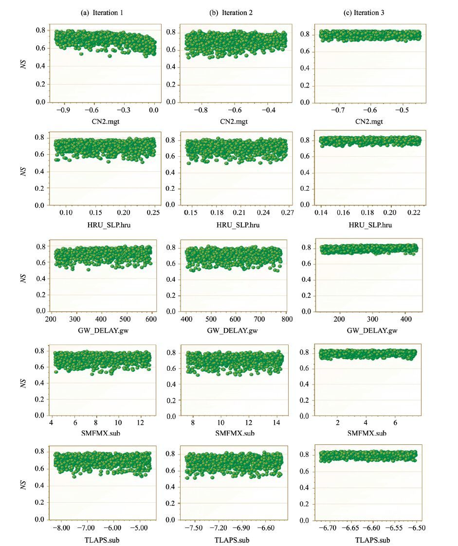
Dot plots (Figure 8) from three iterations, showing parameter values and objective function (NS) values, were also analyzed in this study. The plots present a common challenge of parameter identification, that is, to show the distribution of the sampling points as well as to give an idea of parameter sensitivity (SWAT-CUP, 2015). These plots illustrate that all of our parameters generated a range of values with similar model efficiency, and the equifinality phenomenon was very obvious. Consequently, it was difficult to extract a proper set of parameters from the dot plots. It is evident that the main source of uncertainty resided in the model parameters, but it should be noted that non-identifiability of a parameter does not indicate that the model is not sensitive to that parameter (Shen et al., 2012). Estimation of non-identifiable parameters is difficult as there may be many combinations of all the parameters that would result in a similar model performance. Shen et al.(2012)suggested that instead of a process calibration, the decision regarding modeling could deal with these non-identifiable parameters by setting a confidence interval on the model output.
|
| Figure 8 Dot plots depicting NS against parameter values of the top five sensitive parameters from iterations 1, 2, and 3 |
The dot plots of the top five sensitive parameters, CN2, HRU_SLP, GW_DELAY, SMFMX, and TLAPS, with the parameter ranges against NS values, are shown in Figure 8. It is obvious from the plots that the NS values increased in the second and third iterations; the estimated values of NS in the first, second, and third iterations were 0.78, 0.81, and 0.85, respectively.
It should be noted that in the second iteration, certain parameters had unreasonable ranges and were therefore adjusted for the third iteration. The parameters of the first and second iterations had wide NS ranges of 0.50~0.80. However, in the third iteration this range was reduced to 0.70~0.85, indicating better parameter estimation. However, in the fourth iteration, after 1, 000 simulations, the NS value was reduced from 0.85 to 0.79 because of unreasonable estimation of some of the parameters.
It is worth mentioning here that parameter identification can also be improved by calibration techniques. For example, Yang et al.(2007) used the Generalized Likelihood Uncertainty Estimation (GLUE) and Parameter Solution (PARASOL) techniques of uncertainty analysis, and demonstrated improved parameter identification by the PARASOL technique. Many previous studies have reported on the equifinality phenomenon (wherein different parameter sets result in the same modeling accuracy) using different techniques (e.g., Beven and Binley, 1992; Shen et al., 2012; Xue et al., 2014; Narsimlu et al., 2015; Uniyal et al., 2015). Our results showed that the SWAT model was successfully applied in the study area and reasonably good parameter uncertainty ranges were achieved by using the SUFI-2 method.
5 ConclusionIn this study, the SUFI-2 uncertainty analysis method was used in conjunction with SWAT, a distributed hydrological modeling system for hydrological modeling and quantifying parameter uncertainties in a small watershed of the Soan River Basin in northern Pakistan. The monthly runoff simulation values of R2 and NS during a 10-year calibration period (1991-2000) were 0.91 and 0.85, respectively, and in a 10-year validation period (2001-2010) they were 0.89 and 0.84, respectively, with lower values of PBIAS during both periods. Similarly, the monthly sediment simulation values of R2 and NS for calibration were computed as 0.81 and 0.79, respectively, and for validation they were 0.78 and 0.74, respectively. This demonstrated acceptable simulation performance. Uncertainty results of the SUFI-2 runoff simulation indicated that the 95PPU band could capture more than 70% and 60% the observed data during the calibration and validation periods, respectively. However, the reduction of the p-factor from 72% to 67% indicated large uncertainties, much of it occurring in low-flow predictions during the validation period. For sediment yield calibration and validation, more than 60% of the observed data was captured by the 95PPU band. Further analysis of dot plots of the top five parameters in three iterations indicated that the model efficiency improved in all the iterations and there was better parameter estimation in the last iteration. Our results also indicated that although accurate calibration of certain parameters in this study might not be feasible due to difficult field access, multiple possible values of other parameters might generate similar model efficiency due to the equifinality phenomenon. In this study the SWAT model produced good results with reasonably good parameter uncertainty ranges, meaning this model can be used for further analysis of runoff and sediment load estimation in the study area.
Acknowledgments:The research work was supported by the Centre of Excellence in Water Resources Engineering,University of Engineering and Technology Lahore,and local authorities in Pakistan. The authors would like to express appreciation to the Pakistan Meteorological Department (PMD) and the Capital Development Authority (CDA),Islamabad,for providing valuable data to conduct this research.
| Abbaspour KC, van Genuchten MT, Schulin R, et al, 1997. A sequential uncertainty domain inverse procedure for estimating subsurface flow and transport parameters. Water Resources Research, 33(8): 1879–1892. doi: 10.1029/97WR01230 |
| Abbaspour KC, Yang J, Maximov I, et al, 2007. Modelling hy-drology and water quality in the pre-alpine/alpine Thur water-shed using SWAT. Journal of Hydrology, 333: 413–430. doi: 10.1016/j.jhydrol.2006.09.014 |
| Behera S, Panda RK, 2006. Evaluation of management alternatives for an agricultural watershed in a sub-humid subtropical region using a physical process based model. Agriculture, Ecosystems & Environment, 113(1-4): 62–72. |
| Beven K, Binley A, 1992. The future of distributed models:model calibration and uncertainty prediction. Hydrological Processes, 6(3): 279–298. doi: 10.1002/(ISSN)1099-1085 |
| Bhuyan SJ, Koelliker KJ, Marzen LJ, et al, 2003. An integrated approach for water quality assessment of Kansas watershed. Environmental Modeling Software, 18: 473–484. doi: 10.1016/S1364-8152(03)00021-5 |
| Choi JY, Engel BA, Chung HW, 2002. Daily streamflow modeling and assessment based on the curve-number technique. Hydrological Processes, 16(16): 3131–3150. doi: 10.1002/(ISSN)1099-1085 |
| Flugel WA, 1995. Hydrological response units (HRUs) to preserve basin heterogeneity in hydrological modeling using PRMS/MMS-Case study in the Brol basin, Germany. Modelling and Management of Sustainable Basin-Scale Water Resources Systems, 231: 79–87. |
| Fontaine TA, Cruickshank TS, Arnold JG, et al, 2002. Develop-ment of snowfall-snowmelt routine for mountainous terrain for the Soil and Water Assessment Tool (SWAT). Journal of Hy-drology, 262(1-4): 209–223. |
| Gassman PW, Reyes MR, Green CH, et al, 2007a. The soil and water assessment tool:historical development, applications, and future research directions. Transactions of the ASABE, 50(4): 1211–1250. doi: 10.13031/2013.23637 |
| Gassman PW, Reyes MR, Green CH, et al, 2007b. The soil and water assessment tool:historical development, applications and future research directions. Transactions of the Asabe, 50(4): 1211–1250. doi: 10.13031/2013.23637 |
| Gong Y, Shen Z, Liu R, et al, 2010. Effect of watershed subdivision on SWAT modeling with consideration of parameter uncertainty. Journal of Hydrologic Engineering, 15(12): 1070–1074. doi: 10.1061/(ASCE) HE.1943-5584.0000283 |
| Green WH, Ampt GA, 1911. Studies on soil physics, 1. The flow of air and water through soils. Journal of Agricultural Sciences, 4: 11–24. |
| Gupta HV, Sorooshian S, Yapo PO, 1999. Status of automatic calibration for hydrologic models:momparison with multilevel expert calibration. Journal of Hydrologic Engineering, 4(2): 135–143. doi: 10.1061/(ASCE)1084-0699(1999)4:2(135) |
| Jajarmizadeh M, Harun S, Ghahraman B, et al, 2012. Modeling daily stream flow using plant evapotranspiration method. In-ternational Journal of Water Resources and Environmental Engineering, 4(6): 218–226. |
| Kaur R, Srinivasan R, Mishra K, et al, 2003. Assessment of a SWAT model for soil and water management in India. Land Use and Water Resources Research, 3: 1–7. |
| Kim NW, Lee J, 2008. Temporally weighted average curve number method for daily runoff simulation. Hydrological Processes, 22(25): 4936–4948. doi: 10.1002/hyp.v22:25 |
| Kim NW, Lee J, 2010. Enhancement of the channel routing module in SWAT. Hydrological Processes, 24: 96–107. |
| Li Z, Xu Z, Shao Q, et al, 2009. Parameter estimation and uncer-tainty analysis of SWAT model in upper reaches of the Heihe river basin. Hydrological Processes, 23(19): 2744–2753. doi: 10.1002/hyp.v23:19 |
| Narsimlu B, Gosain AK, Chahar BR, et al, 2015. SWAT model calibration and uncertainty analysis for streamflow prediction in the Kunwari River Basin, India, using sequential uncertainty fitting. Journal of Environmental Processes, 2: 79–95. doi: 10.1007/s40710-015-0064-8 |
| Neitsch SL, Arnold JG, Kiniry JR, et al. 2005. Soil and Water Assessment Tool-Theoretical Documentation (Version 2005). Grassland, Soil and Water Research Laboratory, Agricultural Research Service and Blackland Research Center, Texas Agri-cultural Experiment Station, Temple, TX. |
| Neitsch SL, Arnold JG, Kiniry JR, et al. 2011. Soil and Water Assessment Tool-Theoretical Documentation (version 2009). TWRI Report TR-406. Texas Water Resources Institute, College Station, pp. 618. |
| Nietsch SL, Arnold JG, Kiniry JR, et al. 2005. SWAT Theoretical Documentation (version 2005). Grassland, Soil and Water Research Laboratory, Agricultural Research Service, Temple, TX. |
| Nyeko M. 2010. Land use changes in Aswa basin-northern Uganda:Opportunities and constrains to water resources management. Ph.D. dissertation, University of Naples Federico Ⅱ. |
| Qiu LJ, Lin ZF, Yen RS, 2012. SWAT-based runoff and sediment simulation in a small watershed, the loessial hilly-gullied region of China:capabilities and challenges. International Journal of Sediment Research, 27: 226–234. doi: 10.1016/S1001-6279(12)60030-4 |
| Qiu Z, Wang L, 2014. Hydrological and water quality assessment in a suburban watershed with mixed land uses using the SWAT Model. Journal of Hydrologic Engineering, 19(4): 816–827. doi: 10.1061/(ASCE) HE.1943-5584.0000858 |
| Rostamian R, Jaleh A, Afyuni M, et al, 2008. Application of a SWAT model for estimating runoff and sediment in two mountainous basins in central Iran. Hydrological Sciences Journal, 53(5): 977–988. doi: 10.1623/hysj.53.5.977 |
| Santhi C, Arnold JG, Williams JR, et al, 2001. Validation of the SWAT Model on a large river basin with point and nonpoint sources. Journal of the American Water Resources Association, 37(5): 1169–1188. doi: 10.1111/jawr.2001.37.issue-5 |
| Schuol J, Abbaspour KC, Srinivasan R, et al, 2008. Estimation of freshwater availability in the West African sub-continent using the SWAT hydrologic model. Journal of Hydrology, 352: 30–49. doi: 10.1016/j.jhydrol.2007.12.025 |
| Setegn SG, Srinivasan R, Dargahi B, 2008. Hydrological modeling in the Lake Tana Basin, Ethiopia using SWAT model. The Open Hydrology Journal, 2: 49–62. doi: 10.2174/1874378100802010049 |
| Shen ZY, Chen L, Chen T, 2012. Analysis of parameter uncertainty in hydrological and sediment modeling using GLUE method:a case study of SWAT model applied to Three Gorges Reservoir Region, China. Journal of Hydrology and Earth System Sci-ences, 16: 121–132. doi: 10.5194/hess-16-121-2012 |
| Singh A, Imtiyaz M, Isaac RK, et al, 2014. Assessing the perfor-mance and uncertainty analysis of the SWAT and RBNN models for simulation of sediment yield in the Nagwa watershed, India. Hydrological Sciences Journal, 59(2): 351–364. doi: 10.1080/02626667.2013.872787 |
| Soil Conservation Service. 1972. Hydrology, National Engineering Handbook, Supplement A, Section 4, Chapter 10. Washington, D.C.:Soil Conservation Service, USDA. |
| Srinivasan R, Ramanarayanan TS, Arnold JG, et al, 1998. Large area hydrologic modeling and assessment part Ⅱ:model ap-plication. Journal of the American Water Resources Associa-tion, 34(1): 91–101. doi: 10.1111/jawr.1998.34.issue-1 |
| SWAT-CUP. 2015. SWAT-CUP:SWAT Calibration and Uncertainty Programms-A User Manual. Eawag Swiss Federal Institute of Aquatic Science and Technology. http://swat.tamu.edu/me-dia/114860/usermanual_swatcup.pdf. |
| Talebizadeh M, Morid S, Ayyoubzadeh SA, et al, 2010. Uncer-tainty analysis in sediment load modeling using ANN and SWAT Model. Journal of Water Resources Management, 4(9): 1747–1761. doi: 10.1007/s11269-009-9522-2 |
| Tolson BA, Shoemaker CA. 2004. Watershed modeling of the Cannonsville basin using SWAT2000:model development, calibration and validation for the prediction of flow, sediment and phosphorus transport to the Cannonsville Reservoir. Technical Report. School of Civil and Environmental Engineering, Cornell University, Ithaca, New York, USA. |
| Tripathi MP, Panda RK, Raghuwanshi NS, 2005. Development of effective management plan for critical subwatersheds using SWAT model. Hydrological Processes, 19(3): 809–826. doi: 10.1002/(ISSN)1099-1085 |
| Uniyal B, Jha MK, Verma AK, 2015. Parameter identification and uncertainty analysis for simulating streamflow in a river basin of Eastern India. Hydrological Processes, 29: 3744–3766. doi: 10.1002/hyp.v29.17 |
| Van Griensven A, Meixner T, Grunwald S, et al, 2006. A global sensitivity analysis method for the parameters of multi-variable watershed models. Journal of Hydrology, 324: 10–23. doi: 10.1016/j.jhydrol.2005.09.008 |
| Vilaysanea B, Takaraa K, Luob P, et al, 2015. Hydrological stream flow modeling for calibration and uncertainty analysis using SWAT model in the Xedone river basin, Lao PDR. Procedia Environmental Sciences, 28: 380–390. doi: 10.1016/j.proenv.2015.07.047 |
| White KL, Chaubey I, 2005. Sensitivity analysis, calibration, and validations for a multisite and multivariable SWAT model. Journal of the American Water Resources Association, 41(5): 1077–1089. doi: 10.1111/jawr.2005.41.issue-5 |
| Williams JR, 1969. Flood routing with variable travel time or variable storage coefficients. Transactions of the ASAE, 12(1): 100–103. doi: 10.13031/2013.38772 |
| Williams JR. 1975. Sediment-yield prediction with Universal Equation using runoff energy factor. In:Present and Prospective Technology for Predicting Sediment Yield and Sources. U.S. Dep. Agr. ARS-S40, pp. 244-252. |
| Wu H, Chen B, 2014. Evaluating uncertainty estimates in distrib-uted hydrological modeling for the Wenjing River watershed in China by GLUE, SUFI-2, and ParaSol methods. Journal of Ecological Engineering, 76: 110–121. |
| Xue C, Chen B, Asce M, et al, 2014. Parameter uncertainty analysis of surface flow and sediment yield in the Huolin Basin, China. Journal of Hydrologic Engineering, 19(6): 1224–1236. doi: 10.1061/(ASCE) HE.1943-5584.0000909 |
| Yang J, Reichert P, Abbaspour KC, et al, 2007. Hydrological modeling of the Chaohe Basin in China:statistical model for-mulation and bayesian inference. Journal of Hydrology, 340: 167–182. doi: 10.1016/j.jhydrol.2007.04.006 |
| Zhang X, Srinivasan R, Bosch D, 2009. Calibration and uncertainty analysis of the SWAT model using genetic algorithms and Bayesian model averaging. Journal of Hydrology, 374(3-4): 307–317. doi: 10.1016/j.jhydrol.2009.06.023 |
| Zhang XS, Srinivasan R, Debele B, et al, 2008. Runoff simulation of the headwaters of the Yellow River using the SWAT model with three snowmelt algorithms. Journal of the American Water Resources Association, 44(1): 48–61. doi: 10.1111/j.1752-1688.2007.00137.x |
 2016, 8


