Probabilistic analysis of embankment slope stability in frozen ground regions based on random finite element method
1 Introduction
In geotechnical practice, the properties of soil samples taken from sites are often measured for the later use in numerical simulations. It has been widely recognized that probabilistic analyses are usually more informative compared to deterministic analyses which are based on the average values of material properties(Phoon and Kulhawy, 1999; Phoon and Ching, 2015). When considering the variability of soil properties, the response of a geotechnical system could be quite different, depending on the distribution and variation characteristics of soil properties. For example, the viewpoint that a slope with a larger factor of safety(FOS)should be safer than a slope with a smaller FOS according to the deterministic analysis could be changed if the variability of FOS is assessed(Krahn, 2004). Hence, performing probabilistic analysis on geotechnical problems is essential for evaluating the potential geotechnical risk. Generally, apart from the FOS, the probability of failure(Pf) and the reliability index(b)can be utilized to assess the risk level. Shinozuka and Astill(1972)may have been the first to combine the Monte-Carlo method with the finite element method for the eigenvalue problems of structure. In their method, the material properties were sampled from the distributions of random variables and then the calculation was carried out based on the deterministic finite element method. Although the Monte-Carlo finite element method(MCFEM)is computationally expensive, it is still widely used as a benchmark method because of its reliability and accuracy provided that a large number of samples are given. Apart from the Monte-Carlo method, there are a lot of probabilistic analysis methods, including the first-order reliability method(FORM) and the first-order second-moment reliability method(FOSM).
In the past decades, it has been witnessed that stochastic or probabilistic finite element methods have been successfully applied to various engineering fields including frozen soils and frozen ground engineering. For example, Anisimov et al.(2002)noticed that the active layer exhibits obvious spatial variability in complex terrain, even within relatively small areas, and proposed a stochastic model and equations to evaluate the probability density function, mean value, variance and higher statistical moments of active-layer thickness(ALT). Qi et al.(2005)derived the stochastic finite element formula based on the first-order Taylor expansion for the temperature field of frozen soil subgrade roadbed, and then conducted the stochastic finite element analysis on temperature field for Beiluhe roadbed section of the Qinghai-Tibet Railway. According to Lai et al.(2008), some mechanical properties of warm frozen clay and warm ice-rich frozen clay exhibit greater uncertainty and instability than frozen clays at colder temperatures so that the deterministic strength and constitutive relationship of these clays may not be appropriate. Furthermore, it was found based on investigations that the Weibull distribution is more appropriate for the strength distribution law of these clays. To evaluate the replacement thickness of in-cuts roadbed in permafrost regions, Wen et al.(2010)put forward a probabilistic approach considering the uncertainty of thermal and mechanical parameters of subgrade soils. Based on the Monte Carlo simulation and the first-order second moment method, the probabilistic analysis was conducted for the replacement thickness. Recently, Wang and Zhou(2013)conducted a probabilistic analysis on the temperature field of seasonal frozen soil by applying the stochastic finite element analysis based on Neumann expansion with the thermal conductivity coefficient and specific heat capacity as random fields. Furthermore, the material properties of frozen soils were modeled with random field and the boundary condition of environmental ground surface was modeled with stochastic process. By using the proposed method, the randomness of temperature field of embankment was analyzed(Wang et al.,2015).
Since ground surface boundary conditions can be directly impacted by climate change, numerous efforts have been made to study the randomness of boundary conditions due to climate change. For instance, to reflect the impact of randomness in air temperature and climate change on the stability of permafrost roadbed, Pustovoit(1997)conducted the roadbed design based on the limit state and reliability theories. Dankers et al.(2010)remarked that even though permafrost is generally highly sensitive to global warming, few studies were devoted to assessing the uncertainties in simulating the permafrost response to climate change. Hence, they aimed at identifying and quantifying the main sources of uncertainty in the simulation of the permafrost response, and applied two approaches to model the uncertainties. By using the probabilistic approaches, Yang and Cheng(2011a, 2011b)conducted a series of studies to predict the impact of climate change on permafrost stability along the Qinghai-Tibet Railway, and attention was particularly paid to the probabilistic prediction on ALT along 1 km of the Qinghai-Tibet Railway. The predictions of ALT in the past 40 years and future 100 years were then compared and verified with the practical monitored results. Furthermore, permafrost stability along the railway was classified according to the distribution and magnitude of thaw settlement. Comparison results show that ALT tends to increase in the long term, while the change of ALT and the distribution of underground ice are believed to be two crucial factors affecting the thaw settlement.
Although uncertainties of frozen soils are more remarkable, less attention has been paid to the stochastic characteristics and analysis of frozen soils, which may be partially attributed to the fact that material/state parameters of frozen soils have greater spatial variability and numerical simulations of frozen soils involve complex thermo-hydro-mechanical(THM)coupling interactions. Hence, this study focuses on the probabilistic analysis of frozen soils and frozen ground engineering, but with a pseudo-coupled numerical approach based on the stochastic finite element method(Chen et al.,2013). This paper develops as follows. In Section 2, the pseudo-coupled numerical approach for frozen soil stability analysis, in which the finite element analysis is firstly conducted for the thermal-hydraulic field followed by the stability analysis with strength reduction finite element method, is briefly reviewed. Section 3 introduces the r and om field discretization approach for material properties utilized in this work. Section 4 provides two slope examples, including one simple slope and one embankment slope for high-speed railway in frozen ground regions. Finally, some concluding remarks are summarized in Section 5.
2 Finite element equations for coupled thermal- hydraulic field
For frozen soils, the total volumetric water content qw is composed of the volumetric unfrozen/fluid water content qL and the volumetric ice content qI, that is,
| ${\theta _w} = {\theta _L} + \frac{{\rho _I^{}}}{{\rho _L^{}}}{\theta _I}$ |
(1)
|
where,
rI and
rL are the density of ice and unfrozen liquid water, respectively. Hence, the mixed-form modified Richards equation for mass transfer without considering vapor flow or evaporation can be expressed as(
Chen et al.,2013),
| $\begin{array}{l}
{{\dot \theta }_w} = {{\dot \theta }_L}\left( h \right) + \frac{{{\rho _I}}}{{{\rho _L}}}{{\dot \theta }_I}\left( T \right)\\
\quad \ = \nabla \cdot \left[ {{{\bf{K}}_h}\left( h \right)\,\nabla \left( {h + z} \right) + {{\bf{K}}_T}\,\nabla T} \right] + s\left( {{\bf{x}},\;t} \right)\\
\qquad \qquad \; \left( {{\bf{x}},\;t} \right) \in \Omega \times (0,\;{t_t}]
\end{array}$ |
(2)
|
in which
Kh(
h),
KT(
h)are the liquid hydraulic conductivity tensor due to pressure head gradient and temperature gradient, respectively; The total head is decomposed into
H =
h +
z with
h and
z as pressure head and elevation, respectively;
s is a sink term. In Equation, the time difference of
qL can be written as,
| ${\dot \theta _L} = \frac{{\partial {\theta _L}}}{{\partial T}}\dot T = m_F^{}\dot T$ |
(3)
|
where,
mF=
qL/
T is defined as the slope of frozen soil characteristic curve. Hence, Equation can be rewritten as,
| $\begin{array}{l}
\frac{{{\rho _I}}}{{\rho _L^{}}}{{\dot \theta }_I} = \nabla \cdot \left[ {{{\bf{K}}_h}\nabla \left( {h + z} \right) + {{\bf{K}}_T}\,\nabla T} \right]\\
\quad \quad + s\left( {{\bf{x}},\;t} \right) - m_F^{}\dot T,\;\quad \left( {{\bf{x}},\;t} \right) \in \Omega \times (0,\;{t_1}]
\end{array}$ |
(4)
|
The energy equation which describes heat transport during transient flow for the variably saturated frozen soil is generally expressed as,
| ${C_s}\dot T - {L_f}{\rho _I}{\dot \theta _I} = \nabla \cdot \left( {{\bf{\lambda }}\,\nabla T - {C_L}{{\bf{q}}_L}T} \right)$ |
(5)
|
where,
Cs and
CL are the volumetric heat capacity of soil and liquid water, respectively,
Lf is the latent heat of fusion of water, and
qL is the liquid water flux vector. SubstitutingEquation into Equation, we get,
| $\begin{array}{l}
{C_s}\dot T - {L_f}{\rho _L}\left\{ {\nabla \cdot \left[ {{{\bf{K}}_h}\,\left( {\frac{{{\rm{d}}h}}{{{\rm{d}}T}}\nabla T + \nabla z} \right)\, + {{\bf{K}}_T}\,\nabla T} \right] + s\left( {{\bf{x}},\;t} \right) - m_F^{}\dot T} \right\}\\
\qquad \qquad \qquad \qquad= \nabla \cdot \left( {{\bf{\lambda }}\,\nabla T - {C_L}{{\bf{q}}_L}T} \right)
\end{array}$ |
(6)
|
Furthermore, the generalized Clausius-Clapeyron(GCC)equation is utilized to remove the dilemma that only one equation can be used to solve two basic unknown variables. Eventually, the finite element formulation of Equation can be derived after applying the Galerkin weighted residual method,
| ${{\bf{\tilde E}}_{}}{\bf{\dot T}} + \left[ {{\bf{M}} - {\bf{Q}} + {L_f}{\rho _L}\left( {{{{\bf{\tilde C}}}_h} + {{\bf{C}}_T}} \right)} \right]{\bf{T}} = {{\bf{b}}_{}}$ |
(7)
|
with ${\bf{\tilde E}}$ for the apparent volumetric heat capacity matrix, ${{\bf{\tilde C}}_h}$ for the characteristic matrix of hydraulic conductivity due to
Ñh, ${{\bf{C}}_T}$ for the characteristic matrix of hydraulic conductivity due to Ñ
T,
M for the characteristic matrix of thermal conductivity,
Q for the matrix due to heat convection of flowing water, and
b for the flux vector attributed to the source/sink, gravity,
Ñh,
ÑT and water heat convection, respectively. Applying the finite difference in time domain followed by the fully implicit integration to Equation, the nonlinear iterative expression for the temperature
T can be derived,
| $\begin{array}{l}
\left\{ {{\bf{\tilde E}} + \Delta t_{n + 1}^{}\left[ {{\bf{M}} - {\bf{Q}} + {L_f}{\rho _L}\left( {{{{\bf{\tilde C}}}_h} + {{\bf{C}}_T}} \right)} \right]} \right\}{\bf{T}}_{}^{\left( {n + 1} \right)}\\
\quad = {\bf{\tilde ET}}_{}^{\left( n \right)} + \Delta t_{n + 1}^{}\,{\bf{b}}_{}^{\left( {n + 1} \right)}
\end{array}$ |
(8)
|
To solve Equation, the Picard iterative method can be utilized(Chen et al.,2012). Once the unknown temperature vector T is solved, the pressure head/suction at each node can be achieved.
3 Random field discretization for material properties of frozen soils
The uncertainty in material properties, geometry and external loads may be observed widely for many engineering problems, while what kind of distribution it follows and what is the degree of variability may distinguish the uncertainties. Random field generation is usually utilized to model the variability of soil properties during the finite element analysis, and the resulting method is commonly called stochastic or random finite element method(Sudret and Der Kiureghian, 2000; Fenton and Griffiths, 2008). With the mean m and the coefficient of variance(COV)or st and ard deviation s for one material property(such as the effective Young's modulus or the strength parameters of soils), the Gaussian random field can be truncated as:
| $\hat R\left( {{\bf{x}},\theta } \right) = \mu \left( {\bf{x}} \right) + \sum\limits_{k = 1}^M {\sqrt {\lambda _i^{}} \xi _k^{}\left( \theta \right)\psi _k^{}\left( {\bf{x}} \right)} $ |
(9)
|
in which
xk(
q)denotes a series of orthonormal r and om variables. Consequently, with Equation, the r and omness and space of random field can be separated. Equation can be solved from theFredholm integral equation for the eigenvalue problem by using the wavetlet transformation, that is
| $\int_\Omega {{\cal C}_R^{}\left( {{\bf{x}}_1^{},{\bf{x}}_2^{}} \right)\psi _i^{}\left( {{\bf{x}}_2^{}} \right){\rm{d}}\Omega _{{\bf{x}}_2^{}}^{}} = \lambda _i^{}\psi _i^{}\left( {\bf{x}} \right),\quad i = 1, \cdots $ |
(10)
|
where,
yi(
x)is a complete orthogonal basis of L
2(
y)which is the vectorial space of real r and om variables with finite second moment(
Sudret and Der Kiureghian, 2000),
li are eigenvalues. Hence, any realization of the r and om field can be expressed over the orthogonal basis. The autocovariance function, which is a symmetric positive definite(SPD)matrix, is generally expressed as,
| ${\cal C}_R^{}\left( {{\bf{x}}_1^{},{\bf{x}}_2^{}} \right) = \sigma \left( {{\bf{x}}_1^{}} \right)\sigma \left( {{\bf{x}}_2^{}} \right)\rho \left( {{\bf{x}}_1^{},{\bf{x}}_2^{}} \right)$ |
(11)
|
in which
r(
x1,
x2)can be calculated with different correlation models such as the exponential model or the exponential square model. For 2D problems, the correlation structures can be written as,
| $\rho \left( {{\bf{x}}_1^{},{\bf{x}}_2^{}} \right) = \left\{ {\begin{array}{*{20}{c}}
\begin{array}{l}
\exp \left( { - \frac{{\left| {x_1^{} - x_2^{}} \right|}}{{l_{cx}^{}}} - \frac{{\left| {y_1^{} - y_2^{}} \right|}}{{l_{cy}^{}}}} \right)\\
{\rm{for exponential type}}{\kern 1pt} \quad \quad \quad \quad \;
\end{array}\\
\begin{array}{l}
\exp \left[ { - \left( {\frac{{x_1^{} - x_2^{}}}{{l_{cx}^{}}}} \right)_{}^2 - \left( {\frac{{y_1^{} - y_2^{}}}{{l_{cy}^{}}}} \right)_{}^2} \right]\\
{\rm{for exponential square type}}
\end{array}
\end{array}} \right.$ |
(12)
|
where,
x1=[
x1,
y1],
x2=[
x2,
y2], and
lc=[
lcx,
lcy] is the correlation length vector. The probability density function(PDF)of a normal r and om variable can be found in many texts, hence it is not repeated here. The lognormal r and om variable may often be encountered, and its PDF is generally expressed as,
| $f_X^{}\left( x \right) = \frac{1}{{\sqrt {2{\rm{\pi }}} \sigma _{\ln X}^{} \cdot x}}\exp \left[ { - \frac{1}{2}\left( {\frac{{\ln x - \mu _{\ln X}^{}}}{{\sigma _{\ln X}^{}}}} \right)_{}^2} \right]$ |
(13)
|
From the population mean value μp and st and ard deviation σp the mean value μlnX and st and ard deviation σlnX of the underlying Gaussian field are computed as,
| $\left\{ {\begin{array}{*{20}{c}}
{\sigma _{\ln X}^{} = \sqrt {\ln \left( {1 + \sigma _p^2/\mu _p^2} \right)} }\\
{\mu _{\ln X}^{} = \ln \mu _p^{} - \frac{1}{2}\sigma _{\ln X}^2\quad }
\end{array}} \right.$ |
(14)
|
Since
μp and
σp may not be available in practice, they can be estimated by(
Santoso, 2011),
| $\left\{ {\begin{array}{*{20}{c}}
{\mu _p^{} \approx \tilde \mu _p^{} = \left( {\sum\limits_{i = 1}^N {x_i^{}} } \right)/N\quad \quad \quad \quad \quad \quad \;\;\;}\\
{\sigma _p^{} \approx \tilde \sigma _p^{} = \sqrt {\left[ {\sum\limits_{i = 1}^N {\left( {x_i^{} - \tilde \mu _p^{}} \right)_{}^2} } \right]/\left( {N - 1} \right)} \quad }
\end{array}} \right.$ |
(15)
|
4 Numerical studies
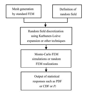
As described above, the coupled thermal-hydraulic field is firstly solved by the 4-node quadrilateral(Q4)finite element method as the numerical accuracy provided by Q4 element should be good enough for this analysis, while the slope stability is analyzed by the shear strength reduction finite element method with 8-node quadrilateral finite elements(Q8)as the Q8 should be more accurate to simulate the stress, strain and displacement fields. For our developed software package "FSoil", the entire computing program is coded in FORTRAN language, and the visualization functions are coded by Python language. To present the probabilistic analysis method utilized in this study, a concise flowchart for the r and om finite element analysis is presented in Figure 1. It is well known that Monte-Carlo simulation is a powerful tool for evaluating the nondeterministic processes of complex systems, and most importantly, it provides a practical approach or a benchmark approach to resolve the problems with high dimensions or vast possibilities, although it is a greedy algorithm(Cipra, 2000). As a result, the Monte-Carlo simulation is utilized for the statistical response of embankment slope.
4.1 Probabilistic slope stability analysis for a homogeneous frozen soil
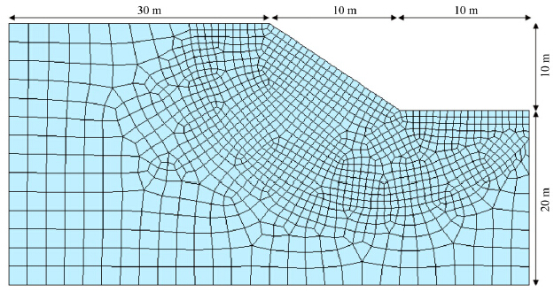
The first slope example, which is composed of 1, 208 elements, has been investigated by Chen et al.(2013), as shown by Figure 2. It is noteworthy that in the present example, the coupled thermal-hydraulic field is not solved so that the strength of frozen soil can't be determined based on the fitted strength parameters, which may depend on temperature and volumetric water(or ice)content(Chen et al.,2013). The soil slope is homogenous except for the cohesion, which follows a normal distribution with the mean as 10 kPa and the COV as 0.3. Hence, the strength variation can be approximately reflected by the normal distribution of cohesion. The Young's modulus E and the Poisson's ratio n are given as 10 MPa and 0.3, respectively. The Mohr-Coulomb soil model with associated plasticity is utilized, and the internal friction angle and the dilation angle are defined as 32° and 32°, respectively. The natural soil weight and saturated soil weight are given as 16 kN/m3 and 18 kN/m3, respectively, and the correlation length along the x and y directions are defined as lcx and lcy, respectively. The effect of correlation length on the r and om field can be observed from Figure 3. It is seen that with an increase of correlation length, the distribution of material property becomes smoother. For the correlation structure, the exponential square model is employed as expressed by Equation .
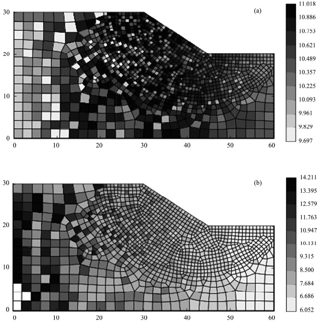
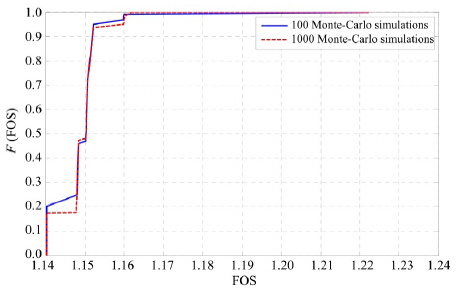
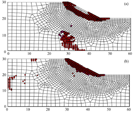
To evaluate the slope, the shear strength reduction finite element method(SSRFEM)is employed and the correlation length lcx = 50 m and lcy = 20 m are applied to generating the r and om field. To accelerate the search process of SSRFEM, the a-algorithm with a taken as 0.2 is utilized to locate the critical(or transition)point between convergence and nonconvergence of the nonlinear Newton-Raphson method. When applying the SSRFEM, the search range for the factor of safety(FOS)is set as [a0, b0] = [0.4, 5.0], and the converged tolerance for the search algorithm of FOS is set as ò= 0.001. To further accelerate the search process of SSRFEM, however, the so-called two-grid search scheme can be used in conjunction with the a-algorithm(Chen et al.,2014a). The Newton-Raphson iteration can be terminated according to the prescribed convergence tolerance tol_nl = 0.01 and the allowable maximum iteration count maxit_nl = 50. For each nonlinear iteration, the symmetric successive over-relaxation preconditioned conjugate gradient(SSOR-PCG)method or the symmetric successive over-relaxation preconditioned symmetric quasi-minimal residual(SSOR-SQMR)method can be adopted(Chen et al.,2006; Chen et al.,2014b). It is noteworthy that in the present slope example, the spatial variability of cohesion of frozen soil is simply simulated with normal distribution, and the effect of thermal-hydraulic field is ignored. In the probabilistic analysis of slope, the Monte-Carlo simulations are performed 100 times and 1, 000 times, respectively, and their cumulative distribution functions(CDF)are plotted in Figure 4. With 100 Monte-Carlo simulations, the calculated mean value and st and ard deviation of FOS are 1.1494 and 0.0088, respectively, while with 1, 000 Monte-Carlo simulations, the calculated mean value and st and ard deviation of FOS are 1.1491 and 0.0055, respectively. Nevertheless, based on the deterministic FEM analysis with constant cohesion(i.e., 10 kPa), the calculated FOS is about 1.7664 which is obviously higher than the probabilistic analysis results, indicating that the probabilistic analysis may provide more information on the slope stability and lead to a more rational design. Hence, based on the 100 Monte-Carlo simulations, it can be concluded that the FOS is 1.1402, 1.1480 and 1.1503 with the confidence of 100%, 79% and 51%, respectively, while based on the 1, 000 Monte-Carlo simulations, the FOS is 1.1402, 1.1480 and 1.1503 with the confidence of 100%, 80% and 51%, respectively. Since the FOS is larger than 1.1402 with the confidence of 100%, we may conclude that the slope will not fail, but the target FOS in the design is 1.1480, we can only say that the slope can meet the design requirement with the confidence of about 80%. The obvious difference in FOS between deterministic analysis and probabilistic analysis may be attributed to the fact that the cohesion of slope may vary in a wide range from 6.052 to 14.211 kPa and slope failure or yielding may occur more easily in those elements with cohesion lower than deterministic value of 10 kPa. As demonstrated by Figure 5 for the distribution of yielding elements, the yielding zone is relatively shallow for the probabilistic analysis compared to the deterministic analysis, since the elements could be weak in strength close to the slope surface as illustrated by Figure 5b. It is noteworthy that there are a few yielding elements distributed scatterly and irregularly, which may contribute to the redistribution of unbalance forces or inaccurate stress integration. However, the existence of these irregularly distributed yielding elements may not obviously affect the observation of slope failure and the accuracy of FOS, and even the scatterly and irregularly distributed yielding elements might be regarded as an indicator that these elements are approaching to the failure stage.
4.2 Probabilistic stability analysis for embankment slope of high-speed railway
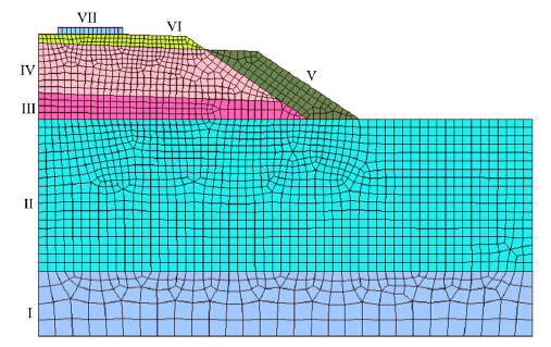
Figure 6 shows the finite element mesh of a typical high-speed railway embankment which is totally composed of seven different materials, including ground soil layers I and II of silty clay, the bottom gravel layer of embankment III, IV layer for group A and B of non-frost-susceptible soils, the slope protection layer V, VI layer for the graded gravel mixed with 5% cement and track slab VII. The latent heat of fusion of ice is given as Lf = 333.55 kJ/kg; the specific heat capacity of soil solid(or particle), liquid water, water vapor and ice are given as 0.8, 4.2, 1.85 and 2.06 kJ/(kg×K), respectively, although they may vary with the environmental temperature; the other hydraulic and strength parameters are given in Table 1. The parameter values are carefully selected by referring to the practical soil materials. To be concise, refer to Chen et al.(2013)for the interpretation of other parameters in Table 1. Before conducting the stability analysis of frozen soil slope, the shear strength of frozen soils has to be defined. There are various shear strength expressions for frozen soils, but the linear Mohr-Coulomb yield criterion, which depends on ice content(or total water content) and temperature, is employed(Chen et al.,2013).
Table 1 Hydraulic and strength parameters of embankment materials
| |
| Soil No. | Hydraulic parameters(van Genuchten) | | Soil strength |
| Empirical parameter, av(m−1) | Empirical parameter, nv(or mv) | Saturated volumetric water content, qs | Residual volumetric water content, qr | Saturated hydraulic conductivity, ks(m/s) | | Cohesion, c(kPa) | Internal friction angle, f(°) |
| I | 1.0 | 1.52 | 0.36 | 0.17 | 1E-6 | | 16.5 | 16.8 |
| II | 1.0 | 1.52 | 0.36 | 0.17 | 1E-7 | | 18.0 | 20.0 |
| III | — | — | — | — | 1E-4 | | 44.2 | 41.5 |
| IV | 1.0 | 1.52 | 0.38 | 0.19 | 1E-7 | | 30.6 | 35.2 |
| V | — | — | — | — | 1E-6 | | — | — |
| VI | — | — | — | — | 1E-4 | | 80.0 | 41.5 |
| VII | — | — | — | — | 1E-11 | | — | — |
| Referring to Figure 6, Soil I and Soil II are natural silty clays; Soil III is the filling gravel; Soil IV is the non-frost-susceptible soil of group A and group B; V is the slope protection structure; VI is the graded gravel mixed with 5% cement; VII is the track slab. |
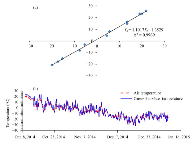
As we know, the ground surface temperature(i.e., Tg)is coupled with the air temperature(i.e., Ta), and generally, it may be simplified to a simple linear relationship, that is,
| $T_g^{} = a \cdot T_a^{} + b$ |
(16)
|
where,
a and
b are coefficients which have to be defined according to practical measurements. According to the measured relationship between ground surface temperature and air temperature in northeastern China(
Wang et al.,2012), the fitted coefficients for Equation are derived as
a = 1.10 and
b = 1.35, as presented in
Figure 7a. Consequently, the ground surface temperature is obtained based on air temperature according to Equation, as presented in
Figure 7b.
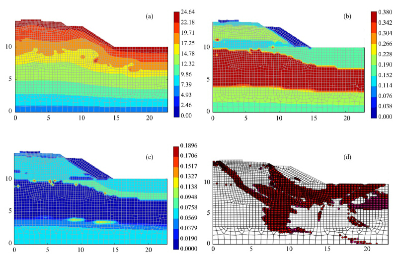
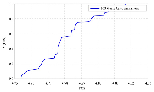
From an initial thermal-hydraulic state, the thermal-hydraulic field is calculated for the starting time(i.e., Oct. 8, 2014)based on the deterministic finite element method. In Figure 8, the temperature field, field of volumetric unfrozen water content, field of volumetric ice content and yielding zone are provided, respectively. It is seen that due to the significant difference in thermal or hydraulic properties of embankment materials, the distinctions of contour between different zones are clear. Based on the derived thermal-hydraulic field, the stability of the embankment slope is analyzed using the SSRFEM and the resultant FOS is about 4.805. The yielding zone in Figure 8d may indicate that the embankment slope may potentially fail from the top point of slope protection contacting the embankment or from the internal edge of track slab. The uncertainty of hydraulic permeability of zone IV may lead to the uncertainty of temperature field and the hydraulic fields, and as a result, lead to the uncertainty of strength parameters of frozen soils and the uncertainty of embankment stability. To determine the variability of soil properties and relevant statistic quantities, we refer to Phoon and Kulhawy(1999) and Phoon and Ching(2015). Figure 9 shows the CDF of FOS due to the lognormal distribution of hydraulic permeability of zone IV with the COV as 0.8. Similar to the slope example in Subsection 4.1, the average value of FOS from 100 simulations(i.e., 4.781)is still smaller than the deterministic analysis(i.e., 4.805), which is similar to the situation of example 1 since the smaller FOS is attributed to the existence of some weak elements.
5 Conclusions
In geotechnical practice, soil sample properties taken from sites are often measured for numerical simulations. It has been widely recognized, however, that probabilistic analyses are usually more informative compared to deterministic analyses which are based on the average values of material properties. In this study, the Monte-Carlo r and om finite element method is utilized to perform the probabilistic analysis on two slope examples, including one simple example and one embankment slope of high-speed railway in frozen ground regions. Numerical results indicate that the distribution of FOS could be more informative than the FOS obtained from the deterministic finite element method since the average of the Monte-Carlo results could be obviously smaller than the deterministic result. In addition, slope failure could be different for probabilistic analysis and deterministic analysis. For example, the slope failure appears to be shallower according to the probabilistic analysis.
Acknowledgments:
This research is supported by the National 973 Project of China(No. 2012CB026104) and the National Natural Science Foundation of China(No. 51378057).
 2015, 7


